
University of Wisconsin Milwaukee University of Wisconsin Milwaukee
UWM Digital Commons UWM Digital Commons
Theses and Dissertations
May 2024
SHORELAND DEVELOPMENT AND DISTURBANCES: A HEDONIC SHORELAND DEVELOPMENT AND DISTURBANCES: A HEDONIC
ANALYSIS OF LAKEFRONT PROPERTIES IN NORTHEASTERN ANALYSIS OF LAKEFRONT PROPERTIES IN NORTHEASTERN
WISCONSIN, USA WISCONSIN, USA
SUSAN BORCHARDT
University of Wisconsin-Milwaukee
Follow this and additional works at: https://dc.uwm.edu/etd
Part of the Natural Resource Economics Commons, and the Water Resource Management Commons
Recommended Citation Recommended Citation
BORCHARDT, SUSAN, "SHORELAND DEVELOPMENT AND DISTURBANCES: A HEDONIC ANALYSIS OF
LAKEFRONT PROPERTIES IN NORTHEASTERN WISCONSIN, USA" (2024).
Theses and Dissertations
.
3458.
https://dc.uwm.edu/etd/3458
This Thesis is brought to you for free and open access by UWM Digital Commons. It has been accepted for
inclusion in Theses and Dissertations by an authorized administrator of UWM Digital Commons. For more
information, please contact [email protected].
SHORELAND DEVELOPMENT AND DISTURBANCES:
A HEDONIC ANALYSIS OF LAKEFRONT PROPERTIES
IN
NORTHEASTERN WISCONSIN, USA
by
Susan Borchardt
A Thesis Submitted in
Partial Fulfillment of the
Requirements for the Degree of
Master of Science
in Freshwater Sciences
at
The University of Wisconsin-Milwaukee
May 2024
ii
ABSTRACT
SHORELAND DEVELOPMENT AND DISTURBANCES:
A HEDONIC ANALYSIS OF LAKEFRONT PROPERTIES
IN
NORTHEASTERN WISCONSIN, USA
by
Susan Borchardt
The University of Wisconsin-Milwaukee, 2024
Under the Supervision of Professor James Price
Shoreland development, encompassing features like boat lifts, manicured lawns, artificial
beaches, and erosion control measures, offers considerable benefits to property owners.
Nevertheless, this development disrupts natural conditions and is associated with increased
sediment and pollutant loading, which negatively impacts aesthetics, recreation, and habitat for
fish and other aquatic species. This thesis conducts two analyses, which respectively quantify the
benefits of shoreland development to homeowners and evaluate the relationship between
shoreland development and lake water quality. In the first analysis, a hedonic property model is
employed to value shoreland development along Wisconsin inland lakes. The model considers
various shoreland development features, using data from 62 lakes surveyed comprehensively
under the Wisconsin Department of Natural Resources (WDNR) Lake Shoreland and Shallows
Habitat Monitoring Program. Results show positive correlations between sales prices and certain
development features, including artificial beaches, erosion control measures, and structures in the
littoral zone, after controlling for housing characteristics and lake fixed effects. Willingness-to-
pay values for these features are derived from the model; these values can be compared to the
welfare loss stemming from sediment and pollutant loading caused by development to inform
iii
shoreland management decisions. In the second analysis, the effect of shoreland development on
lake water clarity is evaluated. Results show that the extent of shoreland development on a lake
is not significantly correlated with water clarity, after controlling for lake characteristic and
nearby land use.
iv
© Copyright by Sue Borchardt, 2024
All Rights Reserved
v
To
my husband who didn’t tell me that;
going back to school was a
crazy idea.

vi
TABLE OF CONTENTS
SHORELAND DEVELOPMENT AND DISTURBANCES: ......................................................... i
ABSTRACT .................................................................................................................................... ii
LIST OF FIGURES ..................................................................................................................... viii
LIST OF TABLES ......................................................................................................................... ix
LIST OF ABBREVIATIONS ......................................................................................................... x
1. Introduction ................................................................................................................................. 1
2. Hedonic Property Analysis ......................................................................................................... 5
2.1. Introduction to Hedonic Analysis ........................................................................................ 5
2.2. Literature Review ................................................................................................................. 5
2.2.1. Economic Valuation Approaches .................................................................................. 6
2.2.2. Hedonic Property Method ............................................................................................. 8
2.3. Study Area and Data .......................................................................................................... 16
2.3.1. Study Area ................................................................................................................... 16
2.3.2. Housing Data ............................................................................................................... 17
2.3.3. Lake Data ..................................................................................................................... 18
2.3.4. Habitat Assessment...................................................................................................... 18
2.4. Methodology ...................................................................................................................... 21
2.4.1. Theoretical Background .............................................................................................. 22
2.4.2. Hot Spot Analysis ........................................................................................................ 29
2.5. Results ................................................................................................................................ 34
2.5.1. Hedonic Model Results ............................................................................................... 34
2.5.2. Marginal Willingness to Pay ....................................................................................... 37
2.5.3. Robustness Checks ...................................................................................................... 41
2.6. Discussion and Conclusion ................................................................................................ 42
2.7. Future Research .................................................................................................................. 44
3. Lake Water Quality Analysis .................................................................................................... 45
3.1. Introduction ........................................................................................................................ 45
3.2. Literature Review ............................................................................................................... 46
3.2.1. Water Quality Determinants ........................................................................................ 46
3.2.2. Buffer Zones ................................................................................................................ 47
3.3. Data .................................................................................................................................... 48
3.3.1. Land Use/Landcover.................................................................................................... 48
vii
3.3.2. Water Clarity ............................................................................................................... 48
3.3.3. Habitat Assessment...................................................................................................... 51
3.4. Methodology ...................................................................................................................... 51
3.5. Results ................................................................................................................................ 52
3.6. Discussion and Conclusion ................................................................................................ 56
3.7. Future Research .................................................................................................................. 57
4. Conclusion ................................................................................................................................ 58
Bibliography .............................................................................................................................. 61
Appendix ....................................................................................................................................... 66
viii
LIST OF FIGURES
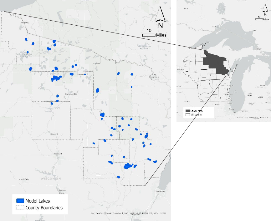
Figure 1 Study lakes and study area for the hedonic models. The size of the study lakes has been
exaggerated for visual clarity. Lake and County shape files were downloaded from the WDNR’s
website (WDNR
2
, n.d.). ................................................................................................................ 17
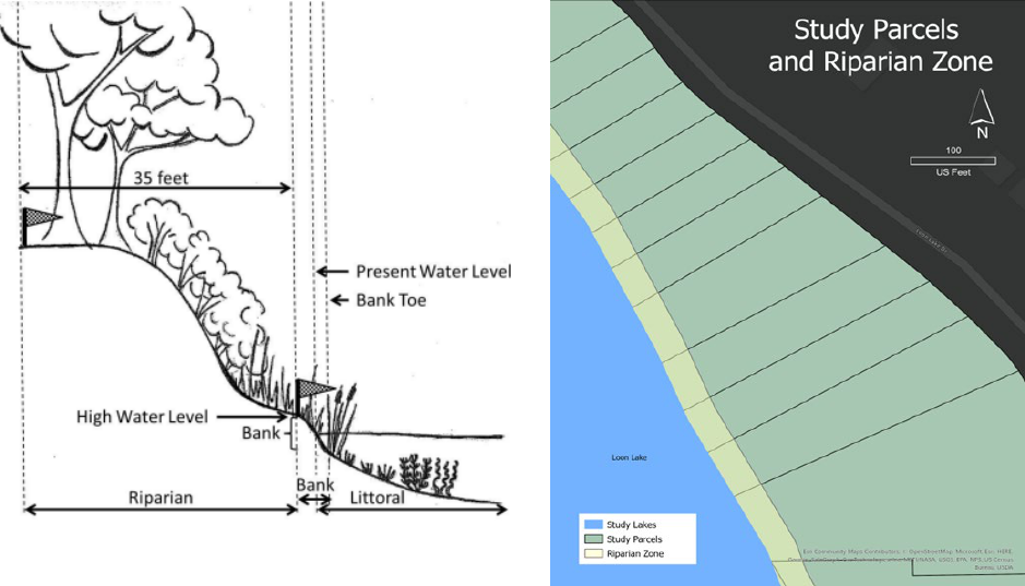
Figure 2 The three habitat zones used in the WDNR Habitat Assessment Study (WDNR, 2020)
....................................................................................................................................................... 20
Figure 3 Plan view of the riparian zone in relation to the study parcels and lakes. Lake shape file
from the WDNR. Parcel shape file from the Wisconsin's State Cartographers Office (n.d.). ...... 20
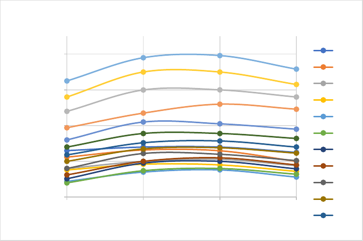
Figure 4 Median sales price of Wisconsin homes from data collected by the Wisconsin Realtors
Association per sales quarter for years 2007-2023, data is updated daily and downloaded from
their website on 2 February 2024 (WRA, 2024) ........................................................................... 27
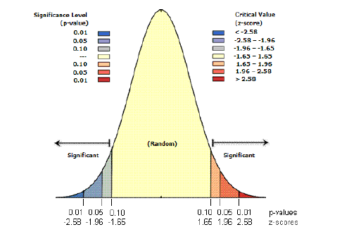
Figure 5 Normal Distribution Curve (ArcGIS Pro, 2023) ........................................................... 30
Figure 6 Hotspots for the variable of the natural log of the quotient derived when the area of the
lot in acres is divided by the length of the shoreline in feet. ........................................................ 33
Figure 7 Hotspots for the variable of the natural log of the home's gross living area in square
feet................................................................................................................................................. 33
Figure 8 Measuring water clarity with a secchi disk, Image from The Many Faces of Water
(Mierzynski, 2017) ........................................................................................................................ 50
Figure 9 Graph of the relationship between the Lakeshore Disturbance Matrix from the
Wisconsin Department of Natural Resources versus the measurement of how deep a secchi disk
can be observed below the surface on 117 Wisconsin lakes. ....................................................... 56
ix
LIST OF TABLES
Table 2.1 Economic Methods for Measuring Environmental and Resource Values
(Tietenberg & Lewis, 2019) .......................................................................................................... 7
Table 2.2. Hedonic Property Model Variable Labels and Descriptions by Variable Type 28
Table 2.3 Model Specifications with Independent Variables Grouped by Variable Type ... 31
Table 2.4 Descriptive Statistics for Variables Used in the Hedonic Property Model ........... 32
Table 2.5 Hedonic Property Model Results (Dependent Variable: Natural Log of Adjusted
Sales Price) ................................................................................................................................... 39
Table 2.6 Overall Model Statistics (Residuals, Degrees of Freedom, F-Stat, and p-value) for
the Five Hedonic Property Models. ........................................................................................... 40
Table 2.7 Marginal Willingness to Pay Per Lakefront Property in Northeastern Wisconsin
(2022 U.S. Dollars) ...................................................................................................................... 40
Table 2.8 Summary of Shoreland Disturbance Results by Shoreland Habitat Zone ........... 41
Table 3.1 Land Use Classes and Descriptions .......................................................................... 49
Table 3.2 Regression Model Specifications for Lake Water Clarity Analysis (Dependent
Variable: Secchi Depth) .............................................................................................................. 52
Table 3.3 Regression Model Results (Dependent Variable: Secchi Depth) ........................... 54
Table 3.4 Overall Model Statistics for Lake Water Clarity Analysis .................................... 55
Table A.1 Robustness Checks for Hedonic Property Model Results (Dependent Variable:
Natural Log of Adjusted Sales Price). ....................................................................................... 66
x
LIST OF ABBREVIATIONS
β
………………..
coefficients
Bypass
………………..
The presence of a feature that allows runoff water to
bypass the filtration effect of the canopy and/or shrubs
Can_Shrub
………………..
Percent of parcel shoreline covered in tree canopy or
shrubs.
CWA
DF
………………..
Clean Water Act
Degrees Of Freedom
EC_Pct
………………..
Percent of parcel shoreline containing artificial erosion
control
EC_Pct
………………..
Percent of parcel shoreline containing artificial erosion
control
ESRI
FRED
………………..
Environmental Systems Research Institute
Federal Reserve Economic Data
GIS
………………..
Geographical Information System
GLA
………………..
Gross Living Area
GS
………………..
number of garage spaces
HPM
………………..
Hedonic property method
HWL
………………..
high-water level
LAKE_NAME
………………..
The name of the lake the property abuts.
LakeA
………………..
Area of the lake in acres
LakeD
………………..
Depth of the lake in feet
LitStruc
………………..
Number of structures in the littoral zone
Ln
………………..
natural log
LnASP
………………..
log of the adjusted sales price of the properties
LnGLA
………………..
natural log of the GLA
LULC
MLS
MMI_L
MMI_P
………………..
Land Use Land Cover
Multiple listing service
Shoreland Habitat disturbance metric per WDNR survey
for the lake as a whole
Shoreland Habitat disturbance metric per WDNR survey
for the parcel as a whole
NR
………………..
natural resources
OHWM
………………..
ordinary high-water mark
P
………………..
property price
r
2
………………..
coefficient of determination
RipStruc
………………..
Number of structures in the riparian zone
RR_Pct
………………..
Percent of parcel shoreline using rip rap for erosion
control
SaleQrt
………………..
The quarter the property sold
SaleYear
………………..
The year the property sold
xi
SD
………………..
Standard deviation
SL
………………..
shoreland length
SWIMS
TWTP
US
Veg
………………..
Surface Water Integrated Monitoring System
Total Willingness To Pay
Unites States
The presence of floating vegetation in the littoral zone
(0,1,2)
VW_Pct
………………..
Percent of parcel shoreline using a vertical wall for
erosion control
WDNR
………………..
Wisconsin Department of Natural Resources
WRA
………………..
Wisconsin Realtors Association
WTP
………………..
Willingness To Pay
x
………………..
property amenities (variables)

1
1. Introduction
Wisconsin is rich in lakes, with over 15,000 documented lakes, of which only about 40% have
been named. Most of the state’s lakes are less than 10 acres, with only 2.4% having a surface
area of at least 20 acres. These larger lakes, however, represent 93% of the approximately one
million acres of surface area that Wisconsin inland lakes cover (WDNR, 2009). All these lakes
mean there is a lot of shoreland in the state, and all this shoreland has been zoned in accordance
with standards established by the Wisconsin Department of Natural Resources (WDNR). The
purpose of shoreland zoning, per the WDNR, is to establish minimum standards to limit the
direct and cumulative impacts of shoreland development on water quality; near-shore aquatic
wetland and upland wildlife habitat; and the natural scenic beauty (WDNR, 2017).
Lakeshore development in Wisconsin began in the 1920s and 30s with the advent of better roads
outside the big cities. Agricultural and forest land abutting freshwater lakes was subdivided into
lots to accommodate small cottages (Yanggen & Kusler, 1968). Cottages usually relied on
outhouses or an onsite septic system, both of which allowed domestic waste to seep into the
ground and find its way to nearby surface water. As demand for proximity to recreational waters
grew, the price of existing lakeshore lots increased, and less desirable lots were developed. The
less desirable lots had steep slopes or were low lying with high groundwater levels, making it
challenging to prevent runoff. This development brought much-needed investment to the rural
communities, but it also increased risks to the natural environment. Uncontrolled development
brought erosion problems from road building and grading and increased runoff from the
displacement of shoreland cover and habitat with manicured lawns and impervious surfaces.
2
To protect the waters and natural beauty of the state's shoreland, Wisconsin enacted its original
shoreland zoning laws in August of 1966 (Yanggen & Kusler, 1968). The WDNR has set
minimum standards that the local zoning authorities can make more, but not less restrictive.
Minimum zoning standards for shorelands are outlined in Chapter NR 115.05 of the Wisconsin
Administrative Code (WDNR, 2017). There are minimum standards for lot size, building
setbacks, vegetation, filling and dredging, use of impervious surfaces, structure height, and the
use of nonconforming structures. There is also a provision that these minimum standards become
the zoning regulation in the case that the county fails to provide zoning standards that meet the
minimums set forth by the WDNR.
The shoreland area, as defined by the WDNR, is land within the following distances from the
ordinary high-water mark (OHWM) of navigable waters: 1,000 feet from a lake, pond, or
flowage; and 300 feet from a river or stream or to the landward side of the flood plain, whichever
distance is greater. The OHWM is the point on the shore where the presence and action of the
water is so continuous as to leave a distinct mark. There are several approved uses of shoreland
property, including parks, agricultural crops, hunting, pasturing of livestock, and both residential
and commercial activities (WDNR, 2017). The zoning laws restrict what an individual property
owner can build or how they can landscape the lot along the shoreline. The ordinances mitigate
negative impacts of development on Wisconsin surface waters by limiting pollution, preserving
fish habitat, and attracting recreation; they are intended to enhance the beauty and value of the
properties with lake frontage (WDNR, 2017). That said, regulations can have a positive or
negative effect on the property’s value. Regulations that put limits on a property's use, or that
limit either directly or indirectly what improvements can be added to the property, can
substantially diminish the land value (Yanggen & Kusler, 1968), while good water quality has
3
been related to a higher value for lakeshore property in studies by Guignet et al. (2022) and
David (1968).
Despite these standards, there is growing recognition of the need for greater shoreland protection
and restoration; these areas are increasingly recognized as critical habitats for fish of both
ecological and economic importance. Shoreland areas are found to be highly productive habitats
that are favored by juvenile fish because they provide refuge from predation and are thus
considered fish nurseries by ecologists (Munsch et al., 2017). It is estimated that recreational
anglers in Wisconsin annually harvest for food ≈ 4,200 metric tons of fish from ≈ 4,000 inland
lakes (Embke et al., 2020). This estimate, derived from creel surveys, does not include the added
impact from the sport of catch and release fishing. Shoreland habitats, however, are being
transformed to support the demands of home buyers seeking lakefront property, and many of
these shorelands are being modified by armoring (artificial erosion control, vertical walls, rip
rap, etc.) and the addition of structures in both the riparian and littoral zones that further facilitate
waterfront use (Munsch et al., 2017). Per Munsch (2017), “these modifications affect the ecology
of nearshore systems by restructuring, eliminating, and shading shallow waters.”
This thesis conducts two analyses, which respectively quantify the benefits of shoreland
development to homeowners and evaluate the relationship between shoreland development and
lake water quality. The first analysis estimates the value homeowners place on characteristics of
shoreland zoning area—considered by the property owner as improvements but as disturbances
by the WDNR—by evaluating variations in property sales prices. When studies are performed
for a housing market, the sales prices vary with access to various amenities and disamenities. For
example, lakefront properties sell for more than similar properties farther away from the water
body, reflecting the homeowners’ willingness to pay (WTP) for the recreational and aesthetic
4
benefits of lake access. The recreational and aesthetic benefits are not traded directly in the
market; they are a non-market good. Economists have developed an analytical model to derive
the customer's WTP for this non-market good called the hedonic property method (HPM)
(Rosen, 1974; Champ et al., 2003; Lansford, & Jones, 1995). The HPM has been used to
evaluate a wide range of environmental amenities, including numerous studies that have
estimated WTP for improved water quality. Few studies, however, have evaluated shoreland
habitat condition or environmental zoning. In this analysis, an HPM is employed to value
shoreland development along Wisconsin inland lakes. Shoreland data are obtained from the
WDNR, which has systematically documented shoreland habitat disturbances at numerous
Wisconsin lakes under the WDNR Lake Shoreland and Shallows Habitat Monitoring Program. A
summary of this work is available on their dashboard (WDNR
1
, n.d.). The HPM in this study
considers various shoreland features, using data from 62 of the surveyed lakes, matched to
household sales data.
Results from the two analyses provide insight into the benefits and costs of shoreland
preservation and restoration efforts in Wisconsin. On one hand, findings from the HPM show
that homeowners place considerable value on some shoreland features, including beaches,
erosion control measures, and recreation-related structures like boat houses. But on the other
hand, the second study on water clarity does not find evidence that shoreland disturbances affect
water clarity. Since the model has a small sample size and is subject to potential omitted
variables bias, this result may not accurately reflect the relationship disturbances and water
clarity. Nevertheless, findings emphasize the need to develop shoreland policies that balance the
benefits and cost of shoreland development.
5
2. Hedonic Property Analysis
2.1. Introduction to Hedonic Analysis
Water frontage, in general, is considered a desirable amenity, whether on a lake, stream, or pond.
As a result, properties that are adjacent to or near a water body have higher sales prices than
other properties, all else equal (Nicholls & Crompton, 2018). But characteristics of the frontage
must also be taken into consideration. Is there a manicured lawn, a vertical wall, or native shrubs
and herbaceous plants at the water’s edge? Are there accessory structures or impervious
surfaces? Is there a dock or an artificial beach? These features affect the benefits homeowners
receive from their shoreland. Shoreland development in the eyes of property owners means
shoreland improvements (manicured lawns, a dock, a boat lift, a swim raft, etc.) that can enhance
recreational and aesthetic benefits of lakefront property. These same improvements, from the
perspective of the WDNR, are shoreland habitat disturbances that negatively impact overall lake
conditions through increased runoff of sediment, nutrients, and contaminants. An improved
understanding of both the benefits and costs associated with shoreland development is essential
for making informed, efficient management decisions.
2.2. Literature Review
The literature review will examine both economic valuation approaches in general and the
specific application of the HPM to water quality and shoreland features. This review will
highlight research gaps within the literature relating to lakeshore habitat and property values.
6
2.2.1. Economic Valuation Approaches
Economists have developed methods for estimating the economic value of both market and non-
market goods and services. Market goods are those goods and services that can be traded in
markets, such as food, shelter, and transportation. Non-market goods, on the other hand, are
those goods and services that are not typically traded in markets, such as scenic views, species
diversity, and clean water (Champ et al., 2003). These goods lack a market price, yet they often
possess substantial economic value.
The environmental amenities (or goods) that are the focus of this study are examples of non-
market goods that are not traded in the traditional market. The total economic value of an
environmental good is made up of three main components: non-use, use, and option values
(Tietenberg & Lewis, 2019). Non-use values include bequest value (saving for future
generations) and existence value (just knowing the item exists with full knowledge that you will
never see or use it). The use value is the benefit a person derives by using the good or service,
which is further divided between consumptive use and non-consumptive use. Consumptive use is
that which diminishes the good through use, such as harvesting fish, while non-consumptive use
does not diminish the good, such as the scenic view of the lake. Option value pertains to saving
goods for possible use in the future. Economists have several methods to estimate the value of
non-market goods (Table 2.1).

7
Table 2.1 Economic Methods for Measuring Environmental and Resource Values
(Tietenberg & Lewis, 2019)
Methods
Revealed Preference
Stated Preference
Direct
Market Price
Contingent Valuation
Simulated Markets
Indirect
Travel Cost
Choice Experiments
Hedonic Property Values
Conjoint Analysis
Hedonic Wage Values
Attribute-Based Models
Avoidance Expenditures
Contingent Ranking
These valuation methods can be divided into two types: revealed preference and stated
preference methods. Stated preference methods are based on hypothetical markets, rather than
real markets. These methods use survey techniques to elicit individuals’ replies within a
structured questionnaire. The survey answers are then used to assess respondents’ willingness to
pay (WTP) for an environmental good or service (Tietenberg & Lewis, 2019). Choice
experiments, conjoint analysis, attribute-based models, and contingent ranking models are
examples of stated preference methods (Table 2.1).
On the other hand, revealed preference methods are based on actual human behavior, where
resource values are inferred from a related marketable good as both goods are internally linked
(Tietenberg & Lewis, 2019). Travel cost, hedonic property or wage values, and avoidance
expenditure models are examples of revealed preference methods (Table 2.1).
In this study, I use a hedonic model to value shoreland conditions, which are environmental
amenities or disamenities that do not have a market value. This method estimates the value of
amenities to homeowners as embodied by the price of the property, thus only the owners’ use
8
value is quantified. To estimate the total recreational and aesthetic value of the shoreland habitat,
other components would need to be added (Lansford & Jones, 1995). To get closer to the total
value, the following also need to be considered: 1) the value of the shoreland to persons living
outside the area who travel to the lake for recreation and 2) value for the existence, bequest, and
option values that persons who will never visit the lake, but who do place a value on its
shoreland habitat (Lansford & Jones, 1995).
2.2.2. Hedonic Property Method
2.2.2.1. Introduction
The hedonic method of estimating WTP is a revealed preference method that uses multiple
regression to discover the environmental component of value (Tietenberg & Lewis, 2019). This
component of value is a use-value of the homeowner, not the general public. The hedonic model
allows for the measurement of the owner’s marginal WTP for marginal changes in individual
attributes (Tietenberg & Lewis, 2019). The HPM has been used widely in different studies
relating to the value of real estate (David, 1968; Gibbs et al., 2002; Young, 1984; Cordell and
Bergstrom, 1993; Loomis and Feldman, 2003; Kashian & Winden, 2020).
Lakes provide numerous benefits to society, including reduced flooding, biodiversity, and non-
use values (Netusil, 2005). The hedonic method provides a means for quantifying these benefits.
Lakes are also a source of recreation-based income that sustains small-town economies,
including many communities in northern Wisconsin (Macbeth, 1989). But Dziuk and Heiskary
(2003, p. 23) put it simply when they stated, “Those who do not fully appreciate the beauty and
recreational use of lakes may find the substantial income from lakes to be adequate justification
for keeping them in a healthy state.”
9
The change in property value as related to a change in water quality or proximity to shoreline has
been studied by several researchers. In Wisconsin, early work by David (1968) examined which
attributes of Wisconsin lakes attributed to increased property values for lake property. The study
took as a given that a customer’s WTP was greater for property that had lake access versus one
that did not. Lakes that were either swampy or had steep slopes had a significant negative
relationship with property values; while good water quality, high surrounding population, and a
higher number of nearby lakes had a significant positive relationship with property values
(David, 1968). There was not a statistically significant relationship between sales prices and road
access to the property, the amount of public land nearby, or the fluctuation of the lake level
(David, 1968). More recent studies, however, have found a significant correlation between lake
level fluctuation and property values (Cordell and Bergstrom, 1993; Loomis and Feldman, 2003;
Kashian & Winden, 2020).
The HPM was chosen for this study because the shoreline characteristics mostly affect the
property owner’s wellbeing, the hedonic method is appropriate for estimating these values.
Moreover, it is likely that most of the use-value of smaller lakes accrue to nearby residents,
rather than to people traveling for recreation. The remainder of this section will discuss how the
HPM has been used to determine WTP for variables relating to shoreland development, water
quality, lake proximity, and lake levels.
2.2.2.2. Shoreland Development
Shoreland development has been linked to changes in shoreland habitat and water quality.
Studies have looked at how Wisconsin’s shoreland management program (the nation’s first) has
affected lake shore aesthetics and controlled development. Nicholls & Crompton (2018), in their
literature review of 47 publications relating to the effects of the proximity and views of inland
10
lakes, found that studies consistently found water views and access were both capitalized into
residential property values. These studies reinforce the DNR’s statement that the purpose of
shoreland development regulations is to maintain safe and healthful conditions; prevent and
control water pollution; protect spawning grounds for fish and other aquatic life; control building
sites and the placement of structures and land uses. The regulations are also in place to preserve
shore cover and natural beauty (WDNR, 2017), which agrees with Klessig (2001) who stressed
both the spiritual, cultural, and emotional value of lakes. To put it simply, the WDNR regulations
were put in place to limit the direct and cumulative impacts of humans on water quality and
aquatic life (WDNR, 2017). Also in Wisconsin, Papenfus & Provencher (2005) in a hedonic
analysis in Vilas County, found that the county's shoreland zoning restrictions requiring
minimum shoreland frontages that were stricter than the state requirements, enhanced property
values. A study in Portland, Oregon, that studied the relationship between environmental zoning
and property values found that the net effect of environmental zoning on a property’s value was
dependent on the type of zoning and the property's location (Netusil, 2005).
In another Wisconsin lakes study, Jennings et al. (2003) found that the quantity of woody debris,
emergent vegetation, and floating vegetation decreased as the density of lakeshore development
increased and that littoral sediments contained more fine particles at these more densely
populated locations. Jennings et al. (2003) goes on to state, “When human activity changes the
physical structure of the environment, it alters the habitat within the lake.” Researchers have
found that by restoring shoreland complexity and minimizing the shade created by structures in
the littoral zone, shoreland habitats that have been compromised by human disturbances can be
restored (Munsch et al., 2017).
11
In nearly the same region as this current study, the northern forested region of Wisconsin,
Horsch & Lewis (2009) found, using information from 170 lakes, that the presence of the
common aquatic invasive species Eurasian Watermilfoil reduced property values by 13%. In the
same study, using the hedonic method they also found that lakes were more likely to be invaded
with the invasive milfoil if it is popular with recreational boaters (Horsch & Lewis, 2009).
Clapper and Caudill (2014) completed a study in Ontario, Canada, which found that the
shoreland length was positively correlated with lakefront cottage values. If that shoreline is
protected with erosion control measures such as a sea wall or rip rap, the value of the property is
increased by 10 percent per Jin et al. (2015), and Mooney and Eisgruber (2001) found that trees
in the riparian zone decrease property values by approximately 3%. This decrease was found
despite the fact that tree cover provides both shade and filtration. Trees slow surface runoff, and
the sediment carried by the runoff is filtered out before it is carried into the lake by the tree’s root
system. They attribute the decline in value to the decreased view of the waterfront (Mooney and
Eisgruber, 2001). While Netusil (2005), on the other hand, found that tree canopy was not
significantly correlated with property values.
Heinrich & Kashian (2010) found that although lake frontage had a positive effect on the price of
homes in rural Wisconsin, the impact was less noted on shallower lakes. These shallower lakes
usually contain more vegetation in the littoral zone due to sunlight being able to reach the lake
bottom of the shallower waters. Gibbs et al. (2002) found that lakes with a larger surface area
were related to higher property values. It is common knowledge in real estate that homes on
larger lakes sell for higher prices; larger lakes offer better recreational opportunities than smaller
lakes (Schnaiberg et al., 2002).
12
2.2.2.3. Water Quality
As far back as the early 1970s, we have been aware of the effects of increased runoff of
fertilizers in the form of phosphorus and nitrates in decreasing water clarity and increasing
primary production leading to low oxygen and, in severe cases, fish kills (Schindler et al., 1971).
Several studies have used hedonic techniques to value changes in water quality. Gibbs et al.
(2002) evaluated the effects of lake size and water quality. They found that water clarity was
more important to customers purchasing property on larger surface area lakes in all four markets
that they studied, and that water clarity had a non-linear relationship with price. The other
variables that Gibbs et al. (2002) found significant to the model were age of the structure, gross
living area (GLA), and depending on the market, the distance to lake, density, and tax rate. They
concluded that reductions in lake clarity due to eutrophication reduced property values and in
turn reduced both state and local tax revenues. Walsh (2009) found that water quality not only
affected the value of lakeshore properties but also affected the value of properties in close
proximity to the lake in a declining gradient as the distance to the lake increased.
Young (1984) analyzed the perceived influence of water pollution on seasonal homes on Lake
Champlain in northern Vermont. They used lot size, GLA, quality of construction, presence of a
garage, and presence of a porch, along with water quality factors as determinants of property
value; they found that the presence of a porch actually added substantial value to the property
and was probably acting as a proxy for one or more unobserved amenities. Water quality was
rated from 1-10, with 1 being poor quality and 10 corresponding to excellent quality. The study
found that each point decline in perceived water quality reduced the property’s value by $1,417
or approximately 6.3%. The properties located on the polluted bay with an average water quality
13
rating of 3.4 were 18.8 to 21% lower in value compared to the properties on the lake with an
average water quality rating of 6.4.
Using water clarity in a hedonic model of 113 lakes across the United States, Moore et al. (2020)
found that on average a 0.1-meter change in Secchi depth led to a 1% change in the property
value of homes near the study lakes. While Clapper and Caudill (2014) found that for each
additional foot of water clarity buyers were willing to pay an additional 2% for lakefront
property. In their meta-analysis, Guignet et al. (2022) used data from 36 unique hedonic studies
to determine elasticity estimates based on water quality metrics. The study found that on average
a 1% change in water clarity produced a 0.1167% change in property value. More recent work in
Wisconsin covering over 100 inland lakes by Wolf et al. (2022) found that decreases in water
quality of approximately 24% led to a loss in value of more than $7500 per parcel. While a
national study, also using the hedonic method, found that a 10% increase in water quality led to a
total increase of between $6 and 9 billion in property value (Mamun et al., 2023). While these
studies concentrated on the relationship between water quality and property value, our study
focuses on the lakeshore disturbances that affect water quality, and their relationship with
property values.
2.2.2.4 Lake Proximity
In a recent literature review, Nicholls & Crompton (2018) found that, in addition to lake
frontage, homeowners are willing to pay for views of and proximity to large lakes and reservoirs.
Thus, the economic value of a lake will be severely underestimated if only the WTP of shoreland
property owners is used for valuation. Accounting for the benefits to property owners in close
proximity to lakes adds millions of dollars to lake values (Nicholls & Crompton, 2018). Not only
is there a positive correlation between the lakes and the surrounding properties' values, but there
14
is also a correlation between lake attributes and the surrounding properties. However, there is a
point where the distance no longer matters; Lansford & Jones, (1995) found that the marginal
price of proximity falls at a declining rate and that there was little change beyond approximately
2,000 feet from the lake.
2.2.2.5. Lake Levels
Loomis and Feldman (2003) analyzed the effect of lowered water levels on property prices. They
found that lower water levels lead to mudflats between the property and the lake. These mudflats
were both unsightly and reduced access to the lake for boating and swimming. The lost use of the
amenity associated with the property was related to a reduced property value. Lansford & Jones
(1995) also found that lower lake levels, which exposed debris that would have been covered by
higher lake levels, were correlated with lower property values. Therefore, higher lake levels
increased WTP due to both greater accessibility and greater aesthetic value.
Loomis and Feldman (2003) used the hedonic method to determine the economic benefit of
maintaining a high lake level for a longer period of time frame during the summer recreation
season. They found that the number of bathrooms, distance to lake, feet of exposed shoreline,
garage spaces, proximity to a golf course, lake frontage, interest rate, building quality, and lake
view were statistically significant predictors of sales price. The lot size and GLA were only
significant in some model specifications. The study found that lower lake levels that exposed an
additional ten feet of shoreline were related to a 1% decrease in property value.
Kashian & Winden (2020), controlling for three different time periods on four different lakes,
evaluated the relationship between property appreciation and linear foot of shoreline. Their
model also used lot size/frontage, GLA, number of rooms, powder room, and bathroom as
15
independent variables; only the number of rooms, powder room, and bathroom were found to be
significant. The study concluded that the WDNR’s decision to lower lake levels in Lake
Koshkonong resulted in financial harm to both individual property owners and the surrounding
community.
2.2.2.6. Non-Market Use Value
These studies, most of which used the HPM, only capture the private benefit of the increased
value of each lakeshore property or properties in close proximity to the water body. Lakes also
provide ecosystem services, including reduced flooding, biodiversity, and non-use value, that
benefit society as a whole (Netusil, 2005). Even without taking into consideration the private
benefits and the ecosystem benefits, the recreational income produced by clean lakes sustains
many northern Wisconsin communities (Macbeth, 1989).
The above hedonic studies all find the non-market, non-consumptive use values of lakes and
shoreland amenities. Additional non-use values of water include existence, bequest, and option
values. When these additional non-use values are bundled together, a total non-use value can be
estimated. This non-use value can then be considered in conjunction with the use value to help
policymakers determine the most economical use of a resource. For example, Lansford & Jones
(1995) found that the net present value of water in both municipal and agriculture exceeded the
marginal recreational and aesthetic values derived from the hedonic method alone. Therefore,
they concluded that for a proper comparison, the additional components of non-use values
needed to be added to make a complete assessment (Lansford & Jones, 1995).
16
2.3. Study Area and Data
2.3.1. Study Area
The study area is located in the northeastern section of the state of Wisconsin in the US (Figure
1). Many of the state’s lakes are bordered by residential development both in the form of year-
round homes and seasonal homes. Some property owners around these lakes have made
substantial changes to the lakeshore habitat, while others have left the shoreland in its natural
state. The WDNR completed an extensive inventory of habitat disturbances on 130 lakes
between 2016 and 2020. A lakeshore disturbance as defined by the WDNR is a disruption or
alteration of the near shore environment, that has been determined to affect water quality. The
availability of the habitat data and sales data from the state’s Multiple Listing Service (MLS)
allow for a hedonic analysis to be performed. The 130 lakes cover an area of approximately 167
km
2
(64.5 mi
2
). The shapefile for the lakes was created from a shapefile of all the lakes in
Wisconsin obtained from the WDNR website (WDNR
2
, n.d.). The lakes range in size from less
than 13,000 m
2
(3.2 acres) to over 25,000,000 m
2
(6178 acres). The study lakes represent a total
lake shoreline of approximately 898,000 meters (558 miles), with the smallest being Bahr Lake
with a shoreline of approximately 724 meters (0.4 miles) and the longest being Tomahawk Lake
with a shoreline of approximately 49,800 meters (31 miles). A statewide geospatial database of
parcels was downloaded from Wisconsin’s State Cartographer’s Office website (Wisconsin State
Cartographer, n.d.). Parcel data was filtered for parcels that have shoreline on the study lakes in
ArcGIS Pro from Esri (ESRI, n.d.).
17
Figure 1 Study lakes and study area
for the hedonic models. The size of
the study lakes has been exaggerated
for visual clarity. Lake and County
shape files were downloaded from the
WDNR’s website (WDNR
2
, n.d.).
2.3.2. Housing Data
The housing data was obtained from Wisconsin’s MLS, a database created and maintained by
professional agents, brokers, and other real estate professionals who belong to Wisconsin’s
Realtors Association (WRA, 2024). The database includes details about listed, sold, expired, and
withdrawn properties listed by the members of the WRA from 2001 to 2022. The MLS data also
includes information on lot size, gross living area (GLA), number of bedrooms and bathrooms,
garage spaces, length of water frontage, the size and floor level each of the homes’ rooms are
located, zoning and school district information, the estimated year the home was built and much
more. The data is entered by the listing real estate agent at the time the property is listed for sale,
18
and updated with the sales information when the property is sold. Although the MLS data is
comprehensive, there are instances where data is missing or incorrect. The MLS data was
cleaned of entries with missing data for date of sale, zero or missing bathrooms, or missing GLA
information. The remaining MLS data was matched spatially to the parcel data using ArcGIS Pro
10.8.2 (ESRI, n.d.). The resulting dataset was then further verified by confirming addresses
matched in both sets of data. The resulting merged dataset contained 847 sold parcels on 62
lakes. Shoreland habitat data was then matched to the MLS sales data using the open-source
statistical computer software program R from the R Project website (R, n.d.).
The next step was to mitigate the temporal influences of inflation, unemployment, seasonal sales,
and mortgage interest rates, by adjusting the sales prices using the quarterly housing price index
for the state of Wisconsin from the Federal Reserve Economic Data (FRED, n.d.). FRED is a
publicly available online database containing economic time series data collected from both
government and private sources by the Research Department of the Federal Reserve Bank of St.
Louis.
2.3.3. Lake Data
Lake-specific variables were incorporated into the dataset and used in some model specifications
to control for observable differences in lake amenities. Specifically, lake area, and lake depth,
were added to the data. Both lake depth and surface area were obtained from the WDNR website
(WDNR
3
, n.d.).
2.3.4. Habitat Assessment
Shoreland habitat was assessed by volunteers using the Lake Shoreland & Shallows Habitat
Monitoring Field Protocol (WDNR, 2020). The assessment covered three zones for each parcel
19
on each study lake (Figure 2). The riparian buffer zone begins at the high-water level (HWL) and
extends inland 35 feet (Figure 3). The assessment used the term HWL versus OHWM due to the
potential legal ramifications. The littoral zone extends into the lake from the current water level.
The bank zone lies between the HWL and the bank toe (the place where the lakebed meets the
bank face). A sample of the data sheet the volunteers completed is available in the Protocol
document (WDNR, 2020).
Within the riparian zone, volunteers working under the direction of the WDNR recorded the
percentage of various land cover features; namely, tree canopy, shrubs, impervious area,
manicured lawn, and agricultural land. Percent cover was recorded to the nearest 5% for each
parcel. Volunteers also recorded the number of structures, boats, and fire pits in the riparian
zone, as well as whether the zone contained a point source, channelized flow area, stairway,
sloped lawn, or bare soil area.
In the bank zone, information was obtained on the percentage of the bank with artificial beach,
vertical sea wall, and riprap. The latter two variables are collectively referred to as erosion
control measures. Information on whether the bank was slumping and whether it was more or
less than 1 foot in height was also obtained. In the littoral zone, the number of human structures
was counted, including piers, boat lifts, swim rafts, boat houses, and marinas. The presence of
floating aquatic and/or emergent plants was noted. If the lake levels were lower than normal and
the lakebed was exposed, then observations were made of plants and other disturbances.
Using information from the riparian, bank, and littoral zones, the WDNR calculated a
disturbance index for each property. Specifically, the index was constructed based on the
percentage of manicured lawn, impervious surface, and agricultural land in the riparian zone, the
percentage of altered bank area (i.e., beach and erosion control), and structure density in both the
20
riparian and littoral zones. Properties with larger index values exhibit greater levels of shoreland
disturbance than properties with smaller values (WDNR, 2023). A lake-level disturbance index is
also constructed using shoreland information for all properties on the waterbody (WDNR, 2023).
The volunteers were instructed to circle the lake in a small boat. From the boat the volunteers
took georeferenced photos and recorded observed habitat disturbances for each parcel. Distances
and percentages were visually estimated for each disturbance recorded. Although the volunteers
were instructed to practice their visual perception of distance by calibrating their eyes using
known measured distances, these estimates still have the potential for bias and imprecision. All
visual estimations, particularly those taken from a distance offshore from a small boat are subject
to a degree of subjectivity, leading to imprecision and error.
Figure 2 The three habitat zones used in the
WDNR Habitat Assessment Study (WDNR,
2020)
Figure 3 Plan view of the riparian zone in
relation to the study parcels and lakes. Lake
shape file from the WDNR. Parcel shape file
from the Wisconsin's State Cartographers
Office (n.d.).
20
Incorporating variables from the WDNR shoreland study into the hedonic model allows for a
comprehensive analysis of how various aspects of shoreland habitat impact property values. The
inclusion of riparian-zone variables such as tree canopy percentage, manicured lawn percentage,
presence of bypass features, and number of structures provides insight into the aesthetic and
environmental characteristics of the shoreline. Tree canopy cover, for example, not only
enhances the visual appeal of the property but also plays a crucial role in filtering pollutants in
runoff, thereby improving water quality.
The presence of bypass features like channelized flows or point source outlets may impact water
quality by allowing runoff to bypass shoreland vegetation, potentially leading to decreased
nearshore water quality. Additionally, the percentage of manicured lawn in the riparian zone,
while offering recreational space and aesthetics, may lack the ecological benefits provided by
native plants and shrubs, such as reducing erosion and nutrient loading.
Moving to the bank zone, variables related to the presence of artificial erosion control measures
and artificial beach areas are considered. While erosion control measures like vertical sea walls
and riprap may offer protection to shorelines, they can negatively impact fish habitat and
macroinvertebrate communities. Artificial beach areas provide recreational benefits but may also
homogenize habitats, affecting aquatic species.
In the littoral zone, variables such as the total number of boat houses, piers, floats, and lifts are
included, reflecting the recreational amenities associated with waterfront properties. The
presence of floating or emergent vegetation and evidence of plant removal also contribute to
understanding how shoreline vegetation affects property values.
21
Furthermore, while this study cannot directly evaluate the effects of zoning ordinances on
property values, it can hypothesize that ordinances aimed at improving water quality may
indirectly influence property values by altering recreational and aesthetic benefits. Contrary to
popular belief, restrictive zoning regulations may not necessarily decrease property values, as
they can enhance the environmental quality and attractiveness of shoreland properties in the long
run.
Overall, integrating these variables into the hedonic model provides a nuanced understanding of
how different aspects of shoreland habitat influence property values, balancing aesthetic,
recreational, and ecological considerations. I hypothesize that many of the shoreland
characteristics are positively correlated with housing prices because they enhance recreational
and aesthetic values (e.g., tree canopy, manicured lawn, structures, beach, erosion control).
Conversely, the presence of channelized flows and floating or emergent vegetation is
hypothesized to have a negative correlation.
2.4. Methodology
The goal of this study is to evaluate how various shoreland features affect housing prices using
the HPM and to estimate marginal WTP values for these features. It is assumed that different
shoreland features have diverse effects on property values, just as they have varying impacts on
water quality and near-shore aquatic habitat. In this study, MLS sales data and information from
the shoreland habitat assessments completed by the WDNR are utilized. A theoretical model
used in this analysis is described below.
22
2.4.1. Theoretical Background
2.4.1.1. Linear vs Non-linear Regression Models
The HPM assumes a perfectly competitive market that determines the equilibrium price for a
home (Rahman, 2021). However, homes are not homogeneous; they are comprised of differing
bundles of structural, neighborhood, and environmental amenities whose quantity and quality
can cause variation in property values. In the hedonic model, differences in property values can
reveal the implicit price of non-market amenities. The implicit price for a marginal change in an
amenity (disamenity), the marginal WTP, is equal to the marginal benefit (loss) to the customer
from that change (Rahman, 2021). The sales price for a home can then be expressed as a multiple
regression equation where the sales price is the dependent variable, characteristics of the
property are independent variables, and estimated parameters represent the amount the price
changes given a change in the independent variables, all else equal. These changes can be either
negative or positive.
The hedonic regression model can take a linear form, as in equation 1, or a nonlinear form, as in
equation 2, where some or all of the independent variables are natural log transformed. It can
also take a nonlinear form where both the dependent variable and independent variables are
natural log transformed, as in equation 3. With the natural log (Ln) transformation, the regression
model can account for a nonlinear relationship. Hedonic property models often exhibit nonlinear
relationships between the dependent variables and the independent variables such as square
footage and lot size (Taylor, 2003). For instance, the value of a marginal increase in GLA
declines as GLA increases. The Ln specification can also help stabilize variance (i.e., reduce
heteroskedasticity), linearize relationships, and normalize skewed data, all of which can improve
a model’s performance (Sakia, 1992).
23
P
i
= β
0
+ β
1
X
1
+ β
2
X
2
+ β
3
X
3
+ e Equation 1
P
i
= β
0
+ β
1
ln(X
1
) + β
2
X
2
+ β
3
ln(X
3
) + e Equation 2
lnP
i
= β
0
+ β
1
ln(X
1
) + β
2
X
2
+ β
3
ln(X
3
) + e Equation 3
Where: P = property price
β = coefficients
X = property amenities
e = error term
The preferred model form is context-specific. Young (1984) found that the linear model
(equation 1) had greater predictive ability and produced coefficients with higher levels of
statistical significance, while Loomis and Feldman (2003) found that a non-linear model
performed better. Both studies compared results from linear and non-linear models estimated
with the same data, testing the sensitivity of results to the model form, and evaluating the
appropriateness of the independent variables included in the model.
2.4.1.2. Box-Cox Model
The Box-Cox model can be used to help identify an appropriate model form. Box and Cox
(1964) proposed a nonlinear transformation method that could make model residuals more
normal and less heteroskedastic. The transformation, which can be applied to any set of strictly
positive dependent and independent variables, is in the form of equation 4.
Y
(λ)
= (Y
λ
– 1)/λ Equation 4
While the estimated parameter lambda can take any value, when it is 1 the transformation is
equivalent to using a linear specification, and when it is 0 the transformation is equivalent to a
natural log specification. For this analysis, I estimated the Box-Cox model with transformations
on the sales price and several structural characteristics. Results suggest that a model with a log-
24
transformed dependent variable and log-transformed independent variables is preferred to a
linear model. Thus, this study employed the model form depicted in equation 3, where the
natural log of the dependent variable was regressed against the property amenities, some of
which were log-transformed.
2.4.1.3. Model Variables
Ideally, all determinants would be included in the hedonic model, but such a model would be
unmanageable due to the large number of factors that affect home prices (Young, 1984).
Furthermore, information for many factors is either not available or of poor quality. In this study,
information on the age of the structure was missing for a large portion of the sales transactions,
so it was not used in the model. An additional reason for limiting the number of independent
variables used in the model is multicollinearity, which occurs when two or more variables are
highly correlated. The inclusion of multicollinear variables can increase estimated standard error
and add little to the predictive ability of the model (Young, 1984). For example, Loomis and
Feldman (2003) omitted the number of bedrooms in their hedonic model due to high correlation
with the number of bathrooms and the GLA. The subset of predictors used in the model becomes
proxies for the related unused factors that also contribute to property values (Loomis and
Feldman, 2003).
The dependent variable used in this study is the natural log of the adjusted sale price (LnASP).
The LnASP ranged between 10.15 and 14.56, with a mean of 12.75 and a standard deviation of
0.54 (Table 2.4). Independent variables used in the model can be divided into three broad
characteristics (structural, neighborhood, and environmental) (Rahman, 2021). For structural
amenities, this study used the log of the home’s GLA (LnGLA), the number of garage spaces
(GS), total number of bathrooms (Tot_Bath), the presence of a dishwasher (DshWshr), the
25
presence of a washer (Wash), the presence of a dryer (Dry), the natural log of the area lot area
per GIS (LnAGIS), and the natural log of the ratio of lot area to shoreland length
(LnAcresPerSL). AcresPerSL is similar to the lot size per lake frontage variable found to be
significant in Kashian & Winden (2020). The average property in this study has 1.7 garage
spaces and 1.5 baths; its GLA is 1687 square feet, and it sits on a 1.2-acre lot that has a shorter
shoreline than its lot depth. Approximately 44% of the study properties have a washer and dryer.
The variables chosen for this study are a combination of those found to be significant in previous
literature and those that were found to be complete in the dataset. The statistics for each variable
are listed in Table 2.4.
The neighborhood amenities are controlled for using lake-level fixed effects. Identical properties
on different lakes can sell for a different price due to differences in lake qualities not addressed
in the model (lake area, depth, water quality, fish stocks, etc.). The fixed effects account for the
overall effect of each lake’s characteristics on home prices, assuming lake qualities remain
relatively constant over the study period. Furthermore, because most lakes in the study are small,
the lake fixed effects also control for the location-specific factors like distance to larger
population centers, school district, and nearby environmental amenities. In some model
specifications, the area of the lake in acres (LakeA) and the depth of the lake in feet (LakeD) are
used in place of the lake fixed effects. The area of the study lakes ranges between 13 and 6215
acres, with the average just over 2000 acres. The average lake depth of the study lakes was
between 8 and 84 feet, and the mean average lake depth was just over 32 feet (Table 2.4).
The environmental amenities are obtained from the shoreland habitat assessment. The
characteristics in the riparian zone that were used were the percentage of forested cover
(CANOPY_PCT), the presence of a bypass (Bypass_Pres), the percentage of manicured lawn
26
(LAWN_PCT), and the number of structures (RipStruc). In the bank area, the characteristics that
were used were the percent of the shoreline that contains artificial erosion control (TotalEC_Pct),
the presence of shoreline erosion (EROSION_PRES), and the percent of shoreline that contains
an artificial beach (BeachPerc). Lastly, in the littoral zone, the characteristics used were the
presence of vegetation (Veg_Pres), evidence that vegetation was removed (Veg_Rem), and the
number of structures (LitStruc). The average number of structures in the littoral and riparian
zones is 1.7 and 1.5, respectively. Some model specifications also use a property-level index of
shoreland disturbance developed by the WDNR (MMI_P). This index is created from numerous
shoreline features, where higher values indicate properties with a greater degree of shoreland
disturbance. The index is a sum of the percentages of shoreland disturbances in the riparian,
littoral and bank zones (WDNR
1
, n.d.). The index ranges between 0 and 400, with the average
disturbance being 214.19 and a standard deviation of 112.32.
In addition to the structural, neighborhood, and environmental variables, additional variables
were used to control for time fixed effects. A similar property with the same bundle of attributes
may sell at a different price in the spring than in the fall of the same year or at a different price
the following spring due to demand, interest rates, etc. (Rahman, 2021). These differences can be
seen in Figure 4, which depicts the median sales value of homes in Wisconsin by sale year and
quarter. This study used fixed effects for both the year (SaleYear) and the quarter (SaleQrt) that
the property was sold, determined by the proprietary sales date listed in the MLS dataset. The
independent variables used in this study are listed in Table 2.2, and the descriptive statistics for
each variable are presented in Table 2.4.
27
Figure 4 Median sales price of Wisconsin homes from data collected by the Wisconsin Realtors
Association per sales quarter for years 2007-2023, data is updated daily and downloaded from
their website on 2 February 2024 (WRA, 2024).
2.4.1.4. Model Specifications
This study estimated five different hedonic model specifications. The first model consisted of the
structural variables and the lake, year-, and quarter-fixed effects. The second model used the
structural variables, fixed effects, and the property-level shoreland disturbance index developed
by the WDNR. In the third model, the disturbance index was replaced by the shoreland
characteristics in the riparian, bank, and littoral zones. The fourth model included the same
structural variables and shoreland variables as the third model but replaced the lake-fixed effects
with the lake area and lake depth variables. Lastly, the fifth model is a parsimonious
specification that removes some of the variables that were not statistically significant in the other
specifications. The models were estimated in the program R using lm_robust found in the
estimatr package (R, n.d.), which generates robust standard errors. A list of the variables
included in each model is provided in Table 2.3.
$100000
$150000
$200000
$250000
$300000
1 2 3 4
Median Sales Price in Dollars
Sales Quarter
Median Sales Price of Wisconsin Homes
2007
2008
2009
2010
2011
2012
2013
2014
2015
2016
2017
Sales Year

28
Table 2.2 Hedonic Property Model Variable Labels and Descriptions by Variable Type
Variable Type
Variable
Description
Structural
LnGLA
Natural log of the buildings gross living area in feet
squared
GS
Number of garage spaces
Tot_Bath>2
Presence of more than 2 baths (0 if not present, 1
otherwise)
Tot_Bath2
Presence of 2 baths (0 if not present, 1 otherwise)
Tot_Bath1
Presence of 1 bath (0 if not present, 1 otherwise)
DshWshr
Presence of a dish washer (0 if not present, 1
otherwise)
Washer
Presence of a clothes washer (0 if not present, 1
otherwise)
Dryer
Presence of a clothes dryer (0 if not present, 1
otherwise)
LnAGIS
Natural log of the area of the parcel per GIS in acres
LnAcresPerSL
Natural log of the Parcels area in acres divided by
shore length in feet
Neighborhood
LakeA
Area of the lake in acres
LakeD
Depth of the lake in feet
Environmental
MMI_P
Shoreland habitat disturbance index
CANOPY_PCT
Percent of parcel shoreline covered in tree canopy.
LitStruc
Number of structures in the littoral zone
RipStruc
Number of structures in the riparian zone
TotalEC_Pct
Percent of parcel shoreline containing artificial erosion
control.
EROSION_PRES
Presence of indication of shoreland erosion (0 if not
present, 1 otherwise)
BeachPerc
Percent of parcel shoreline containing artificial beach.
LAWN_PCT
Percent of parcel in the riparian zone containing a
manicured lawn.
Bypass_Pres
The presence of a feature that allows runoff water to
bypass the filtration effect of the canopy (0 if not
present, 1 otherwise).
Veg_Rem
Presence of indication of plant removal activity (0 if
not present, 1 otherwise)
Veg_Pres
The presence of floating and/or emergent vegetation in
the littoral zone (0 if not present, 1 otherwise)
Fixed Effects
Variables
SaleYear
The year the property sold (2001 – 2022)
SaleQrt
The quarter the property sold (1,2,3 or 4)
LAKE_NAME
The name of the lake the property abuts.
29
2.4.2. Hot Spot Analysis
Variation in sales prices and housing characteristics across space is known as spatial
heterogeneity. Anyone working with real estate knows that location matters; the three most
important attributes of real estate are “location, location, location”. The First Law of Geography,
according to Waldo Tobler (1970), is "everything is related to everything else, but near things are
more related than distant things”. This is especially true for property values, where a real estate
professional determines the value of a property by finding nearby properties (location) with
similar attributes to the subject property that have sold recently (time). The professional then
compares these properties to the subject property to make an estimate of its value. Therefore, if
the most important attribute is location, the second most important attribute is time. To evaluate
patterns in spatial heterogeneity in property attributes, I used Hot Spot Analysis.
Hot Spot Analysis can determine if the property characteristics are clustered spatially using the
Getis-Ord Gi* statistic, which is calculated and mapped using the Hot Spot Analysis tool in
ArcGIS Pro (n.d.). The analysis assesses whether high or low values for a variable are
concentrated spatially using the Gi* statistic, which is a z-score (ArcGIS Pro, n.d.).
The G
i
*
statistic looks at each feature within its own neighborhood to determine not only does it
have a high or low value but is it statistically significant. To be significant a feature must not just
be high or low, but it must be surrounded by similarity high or low neighbors. The features
value, along with its neighbors’ values are summed and compared with the proportionate sum of
all the features to determine if the sum is too large or small to be the result of just random chance
(ArcGIS Pro, n.d.).
30
Figures 6 and 7 depict the spatial variation of z-scores for two variables: the natural log of GLA
(LnGLA) and the ratio of lot area to shoreland length (AcresPerSL). These variables were
selected because the size of the home and the length of the shoreline are recognized as two
primary factors influencing a customer’s willingness to pay for lake property in the real estate
industry. The statistics for these variables are detailed in Table 2.4.
The z-scores indicate the number of standard deviations (SD) an observed value deviates from
the mean of the variable's distribution. A z-score falling between ±1.65 and 0 suggests random
attribute variation, resulting in a Gi_Bin or confidence level score of 0. Conversely, if the score
is < -1.65 or > 1.65, the variation is considered significant, leading to a Gi_Bin score ranging
between ± 1 to ± 3. These bins represent the number of SDs the attribute value deviates from the
mean, as illustrated in the example normal distribution curve in Figure 5.
In Figures 6 and 7, the Gi_Bin scores for each parcel are mapped at their respective locations.
Remarkable spatial clustering of property characteristics is observed, both around lakes and
groups of lakes. These findings suggest the presence of unobserved factors related to lakes or
lake groups that may impact sales prices. Hence, this supports the utilization of lake-level fixed
effects in the regression model to account for these factors.
Figure 5 Normal Distribution Curve (ArcGIS Pro, 2023)

31
Table 2.3 Model Specifications with Independent Variables Grouped by Variable Type
Model
Structural
Environmental
Location
Fixed Effects
1
LnGLA
GS
Tot_Bath
DshWshr
Wash
Dry
LnAGIS
LnAcresPerSL
SaleYear
SaleQrt
LAKE_NAME
2
LnGLA
GS
Tot_Bath
LnAGIS
LnAcresPerSL
MMI_P
CANOPY_PCT
Veg_Pres
Veg_Rem
SaleYear
SaleQrt
LAKE_NAME
3
LnGLA
GS
Tot_Bath
LnAGIS
LnAcresPerSL
CANOPY_PCT
LitStruc
RipStruc
TotalEC_Pct
EROSION_PRES
Bypass_Pres
LAWN_PCT
BeachPerc
Veg_Pres
Veg_Rem
SaleYear
SaleQrt
LAKE_NAME
4
LnGLA
GS
Tot_Bath
LnAGIS
LnAcresPerSL
CANOPY_PCT
LitStruc
RipStruc
TotalEC_Pct
EROSION_PRES
Bypass_Pres
LAWN_PCT
BeachPerc
Veg_Pres
Veg_Rem
LakeA
LakeD
SaleYear
SaleQrt
5
LnGLA
GS
Tot_Bath
LnAGIS
LnAcresPerSL
LitStruc
TotalEC_Pct
EROSION_PRES
BeachPerc
SaleYear
SaleQrt
LAKE_NAME

32
Table 2.4 Descriptive Statistics for Variables Used in the Hedonic Property Model
Max.
Min.
Avg.
Std. Dev.
Dependent Variable
LnASP
14.563
10.151
12.748
0.536
Structural Variables
GS
4
0
1.721
1.160
LnGLA
9.055
5.768
7.320
0.466
Tot_Bath
2
1
1.534
0.499
DshWshr
1
0
0.388
0.488
Dry
1
0
0.440
0.497
Wash
1
0
0.445
0.497
LnAGIS
3.959
-2.641
-0.572
0.944
LnAcresPerSL
-1.762
-6.907
-5.118
0.648
Environmental Variables
MMI_P
400
0
214.187
112.315
Veg_Pres
1
0
0.419
0.494
Veg_Rem 1 0 0.152 0.360
CANOPY_PCT
100
0
50.248
35.691
Bypass_Pres
1
0
0.649
0.477
TotalEC_Pct
100
0
34.536
43.842
EROSION_PRES 1 0 0.095 0.293
LAWN_PCT
100
0
56.954
37.462
BeachPerc
100
0
4.317
18.253
LitStruc
8
0
1.721
1.250
RipStruc
17
0
1.543
2.075
Location Variables
LakeA
6215
13
2159.711
2754.362
LakeD
84
8
32.411
10.961
Fixed Effects Variables
SaleYear
2022
2001
2014.64
4.917
SaleQrt
4
1
2.519
1.033
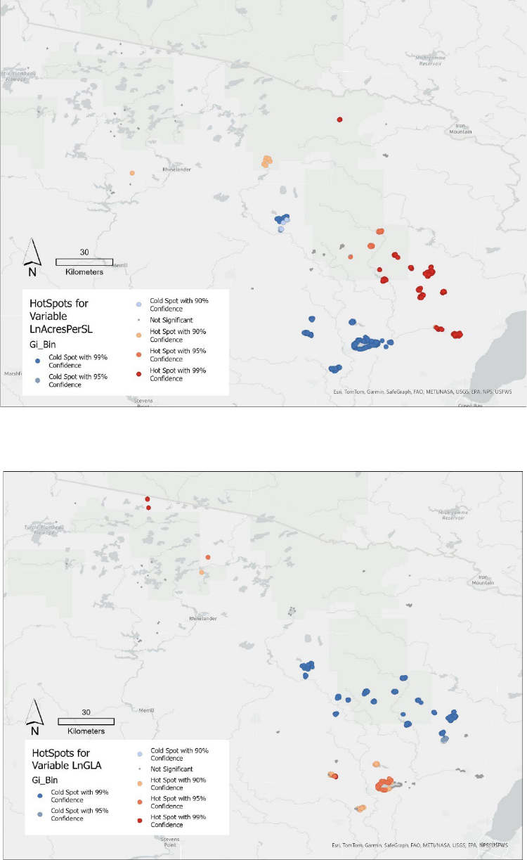
33
Figure 6 Hotspots for the variable of the natural log of the quotient derived when the area of the
lot in acres is divided by the length of the shoreline in feet.
Figure 7 Hotspots for the variable of the natural log of the home's gross living area in square
feet.
34
2.5. Results
This chapter will discuss the results from the five hedonic model specifications (models 1-5). All
five hedonic models used the natural log of the adjusted sales price (LnASP) as the dependent
variable, and all models exhibited statistically significant F-statistics (p-value of 2.2e-16),
indicating that the models provide a better fit to the data than the sample mean.
2.5.1. Hedonic Model Results
Parameter estimates are reported in Table 2.5, and overall model statistics (i.e., error term
distribution, F-statistic) are provided in Table 2.6. A summary of results for shoreland variables
by shoreland habitat zone is provided in Table 2.8. All models contained fixed effects for the
sales year and quarter, while models 1-3 and 5 also included fixed effects for the 62 study lakes.
Models were estimated with robust standard errors in R. At their largest, residuals ranged
between -2.3 and 1.1, with a median value of 0.05. In all five models, the residuals were
approximately normally distributed around 0 without any extreme outliers. The F-Statistics of
models 1-3 and Model 5 ranged between 12.52 and 13.38, with degrees of freedom (DF)
between 746 and 753. Model 4, which did not include the lake fixed effects, had an F-statistic of
18.22 and DF of 805.
The first model (Model 1) included each property’s structural variables and fixed effects for the
year of sale, quarter of sale, and the lake the property was abutting. Model 1 has an r
2
of 0.6205,
meaning that the model explains approximately 62.1% of the variability in the log of property
values. The variables for the presence of appliances (Wash, Dry, and DshWash) are not
statistically significant. However, the variables describing the lot (LnAGIS and LnAcresPerSL)
were both significant, with LnAGIS at p < 0.01 and LnAcresPerSL at p < 0.05. The variable
35
LnAGIS was positively correlated with property value, indicating that larger lots sold for more,
all else being equal. The variable LnAcresPerSL was negatively correlated with property value,
implying that properties with less shoreland per acre sold for less. The variables GS and LnGLA
were also significant at p < 0.01, showing a positive correlation with property value, meaning
that larger homes and homes with more garage spaces had higher sales prices. Homes with more
than two bathrooms (Tot_Bath > 2) also had higher sales prices. The fixed effects accounted for
the differences of both time and location with varying degrees of significance and correlation.
The next model (Model 2) incorporated several environmental variables: each property’s
shoreland disturbance index (MMI_P), the percent of canopy cover (CANOPY_PCT), and the
variables indicating the presence and removal of vegetation in the littoral zone (Veg_Pres,
Veg_Rem). As previously described, the habitat disturbance index is determined using the
percent of the riparian zone that is covered by a manicured lawn, the density of structures in both
the riparian and the littoral zones, and the percent shoreline with bank alterations. The variables
for the presence of appliances (Wash, Dry, and DshWash) were dropped from this model due to
a lack of statistical significance. Model 2 has an r
2
of 0.6204, which is slightly less than the
previous model. Therefore, the addition of the MMI_P variable, along with the canopy and
vegetation in the littoral zone variables, did not meaningfully affect the model’s overall fit to the
data. The adjusted r
2
also decreased from 0.5736 in Model 1 to 0.5729 in Model 2. The adjusted
r
2
makes an adjustment for the number of variables in the model. The MMI_P variable, however,
is statistically significant to the model at p < 0.01 and has a positive correlation with the log of
the property’s value, meaning that properties with greater levels of shoreland disturbance sold for
more, all else being equal. The sign and significance of the structural variables in this model
were similar to those from Model 1.
36
Model 3 replaced the shoreland disturbance index with measures of the index's various
components, while still including variables on canopy coverage and vegetation. The r
2
for Model
3 increased slightly over Model 1, explaining 62.7% of the variability in property value. The
addition of structures in the littoral zone added to the value of lake property at a significance
level of p < 0.05, while the number of structures in the riparian zone was not significant. The
percentage of the shoreline that had erosion control, such as a vertical wall or rip rap, had a
positive effect on value at a significance level of p < 0.01, while the presence of erosion was
negatively correlated with price at p < 0.05. The percentage of the riparian area with tree canopy
and the percentage with manicured lawn was again not significant. The coefficient pertaining to
the presence of a stormwater bypass was negative but also not significant. However, the
percentage of artificial beaches did have a positive and statistically significant effect on property
value at p < 0.05. In the littoral zone, the presence of floating and/or emergent weeds did not
have a significant effect on value, and neither did evidence of the removal of vegetation. The
sign and significance of the structural variables remained unchanged Table 2.5.
In Model 4, lake fixed effects were replaced with variables describing the lake area (LakeA) and
lake depth (LakeD). The fixed effects were removed to evaluate the robustness of results to a
model specification that did not control for location-specific factors, like distance to a larger
population center, school district, and nearby environmental amenities. Without the lake fixed
effects, the r
2
was only 0.4813, effectively reducing the model’s predictive abilities by 15%. The
lake depth and lake area were both significant at p < 0.01. Lake depth was positively correlated
with sales price, while lake area was negatively correlated with the property value. The removal
of the lake fixed effects also affected the significance and magnitude of some of the
environmental and structural variables. Most notably, the lot size and ratio of lot size to shoreline
37
were no longer significant. Moreover, the absolute value of the coefficients for the percentage of
shoreline with a beach, percentage of shoreline with erosion control, presence of a bypass, and
number of structures in the littoral zone increased.
The final model (Model 5) is a parsimonious specification; it is similar to Model 3 but excludes
shoreland variables that were not statistically significant (i.e., LAWN_PCT, CANOPY_PCT,
RipStruc, Bypass_Pres, Veg_Pres, and Veg_Rem). Excluding these variables reduced the r
2
value from 0.6239 to 0.6230, but due to the reduced number of variables, the adjusted r
2
value
increased from 0.5741 to 0.5765. The included structural and shoreland variables are all
significant, and the sign and magnitude of the coefficients are all similar to those in Model 3.
Model 5 is the preferred model specification; it includes those variables that influence the value
of lake shore properties along sampled lakes. The resulting regression equation is:
lnASP = 8.95 + (0.48) LnGLA + (0.07)GS + (0.13)TotBath>2 + (0.09)LnAGIS + (-
0.08)LnAcresPerSL + (0.002)BeachPerc + (0.03)LitStruc + (0.001)TotEC_Pct + (-
0.11)ERSION_PRES0 + β(LAKE_NAME) + β(SaleYear) + β(SaleQrt) + e Equation 5
Where: β = coefficients
LAKE_NAME = Lake fixed effects
SaleYear = Sale year fixed effects
SaleQrt = Sale quarter fixed effects
e = The error term
Results of the five regression runs are shown in Table 2.5. The table consists of the coefficients
and p-values for each variable included in each of the models along with r
2
and adjusted r
2
for
each of the models. The statistics defining the residuals for each of the models are in Table 2.6.
2.5.2. Marginal Willingness to Pay
In Table 2.7, I present the estimated change in the adjusted value of a property given a one-unit
change in an independent variable (i.e., the marginal WTP values). These estimates are based on
38
Model 5 and are calculated using sample averages. The average value of a property in the study
is $392,700.04. Marginal WTP values for the structural variables are reasonable and consistent
with industry norms: an additional square foot of GLA increased the property value by $111.20,
and an additional garage space increased the property value by $26,271.63. Compared to a
property with less than two bathrooms, having more than two bathrooms increased the property
value by $49,126.78. An additional acre in lot size added $31,069.18 to the value of the property.
Most of the shoreland variables were positively correlated with property value, with the
exception of the presence of erosion in the riparian zone, which exhibited a negative relationship.
The presence of erosion decreased the property value by $42,450.87. An additional percent of
artificial beach added $628.32 to the property value. Since the average percent of artificial
beaches is 4.3 percent, artificial beaches add (4.3 * $628.32) $2,701.78 to the value of the
average study property, assuming constant marginal WTP. An additional structure in the littoral
zone adds $11,113.41 to the property value, and each additional percent of erosion control adds
$431.97 to the value. Since the average percent of erosion control per property is 34.5 percent,
erosion control measures add approximately (34.5 * $431.97) $14,902.97 to the value of the
average property. Likewise, the average number of structures in the littoral zone per property is
1.72, and the increase in property value due to these structures is (1.72 * $11,113.41), which is
$19,115.07 for the average property.
Although the amount that the presence of erosion correlates to reduced WTP is high at $-
42,450.87, erosion is only observed at a small fraction of properties, leading to a small effect on
the average property (0.096 * $-42,450.87) at $-4,075.28. In summary, the value added from
features classified as shoreland disturbances is equal to ($2,701.78 + $14,902.97 + $19,115.07),

39
which is $36,719.82 on average for each property, and subtracting the effects of erosion, the total
becomes ($36,719.82 - $4,075.28), which is $32,644.54.
Table 2.5 Hedonic Property Model Results (Dependent Variable: Natural Log of Adjusted
Sales Price)
Variable Model 1 Model 2 Model 3 Model 4 Model 5
LnGLA
0.4847***
(0.0000)
0.4832***
(0.0000)
0.4798***
(0.0000)
0.4324***
(0.0000)
0.4778***
(0.0000)
Garage Spaces
0.0613***
(0.000003)
0.0694***
(0.00000)
0.0657***
(0.000001)
0.0528***
(0.0001)
0.0669***
(0.000001)
Total Bath >2
0.0971*
(0.0821)
0.1211**
(0.0302)
0.1258**
(0.0245)
0.2506***
(0.00003)
0.1251**
(0.0195)
2
-0.0161
(0.6551)
0.0009
(0.9797)
-0.0002
(0.9958)
0.0360
(0.3591)
0.0016
(0.9636)
Presence of a Dryer
0.1080
(0.2020)
Presence of a Washer
-0.0148
(0.8608)
Presence of a Dishwasher
0.0010
(0.9688)
Ln of Lot Acres per GIS
0.0819***
(0.0020)
0.1215***
(0.00003)
0.0973***
(0.0007)
0.0193
(0.4647)
0.0927***
(0.0006)
Ln of Acres/Shore Length
-0.0731**
(0.0431)
-0.1008***
(0.0066)
-0.0916**
(0.0157)
0.0379
(0.2672)
-0.0816**
(0.0247)
Shoreland Metric
0.0004***
(0.0028)
Manicured Lawn Percent
-0.0002
(0.6354)
-0.0003
(0.5805)
Canopy Percent
0.0005
(0.2738)
0.0002
(0.5734)
0.0003
(0.5209)
Beach Percent
0.0017*
(0.0314)
0.0020**
(0.0206)
0.0016**
(0.0241)
Structures Lit Zone
0.0296**
(0.0128)
0.0732***
(0.0000)
0.0283**
(0.0151)
Structures Rip Zone
-0.0052
(0.4819)
-0.0115
(0.1108)
Erosion Control %
0.0012***
(0.0018)
0.0023***
(0.0000)
0.0011***
(0.0022)
Erosion Present
-0.1138**
(0.0120)
-0.1493***
(0.0028)
-0.1081**
(0.0152)
Bypass_Pres
-0.00051
(0.6063)
0.0049
(0.8818)
Vegetation Present
0.0280
(0.3649)
0.0210
(0.5020)
0.0231
(0.4649)
Vegetation Removed Pres
- 0.0070
(0.8632)
-0.0084
(0.8373)
-0.0565
(0.1751)
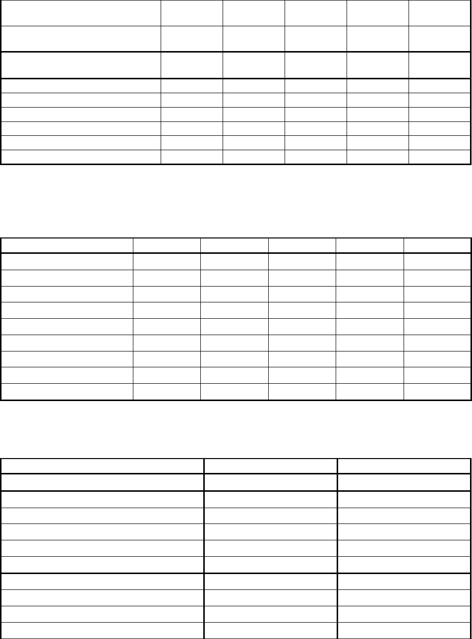
40
Lake Depth
0.0072***
(0.000003)
Lake Area
-0.00002**
(0.0038)
Constant
9.0197***
(0.0000)
8.7218***
(0.0000)
8.8934***
(0.0000)
9.6564***
(0.0000)
8.9529***
(0.0000)
Year fixed effect
Yes
Yes
Yes
Yes
Yes
Quarter fixed effect
Yes
Yes
Yes
Yes
Yes
Lake fixed effect
Yes
Yes
Yes
No
Yes
Observations
847
847
847
847
847
r
2
0.6205
0.6204
0.6270
0.4813
0.6260
Adjusted r
2
0.5736
0.5729
0.5769
0.4548
0.5792
Note: Robust standard errors reported in parentheses.
*p<0.1; **p<0.05; ***p<0.01
Table 2.6 Overall Model Statistics (Residuals, Degrees of Freedom, F-Stat, and p-value) for
the Five Hedonic Property Models.
Statistic
Model 1
Model 2
Model 3
Model 4
Model 5
Residual Min
-2.03476
-2.09613
-2.0811
-2.28197
-2.08227
Residual 1Q
-0.11983
-0.12016
-0.1215
-0.17524
-0.13037
Residual Median
0.03804
0.04247
0.0410
0.04926
0.03814
Residual 3Q
0.19739
0.20149
0.1954
0.23040
0.19638
Residual Max
0.73206
0.79275
0.7957
1.08034
0.79747
Residual Standard Error
0.3499
0.3502
0.3485
0.3957
0.3476
DF
753
752
746
805
752
F-Stat
13.24
13.07
12.54
18.22
13.39
p-value
2.2e-16
2.2e-16
2.2e-16
2.2e-16
2.2e-16
Table 2.7 Marginal Willingness to Pay Per Lakefront Property in Northeastern Wisconsin
(2022 U.S. Dollars)
Variable
Model 5
Ave. Property
ASP
392,700.04
LnGLA
0.4778*** (0.00000)
111.20
Garage Spaces
0.0669*** (0.000001)
26,271.63
Total Bath >2
0.1251** (0.0241)
49,126.78
Ln of Lot Acres per GIS
0.0927*** (0.0006)
31,069.18
Ln of Acres/Shore Length
-0.0816** (0.0247)
-1,791.35
Beach Percent
0.0016** (0.0241)
628.32
Structures Littoral Zone
0.0283** (0.0151)
11,113.41
Erosion Control Percent
0.0011*** (0.0022)
431.97
Erosion Present
-0.1081** (0.152)
-42,450.87

41
Table 2.8 Summary of Shoreland Disturbance Results by Shoreland Habitat Zone
Shoreland Habitat Zone
Environmental Variable
Statistical Significance
(p<0.05)
Littoral
Structures
Yes Positive
Vegetation Present
No
Vegetation Removed
No
Bank
Erosion
Yes Negative
Percent Erosion Control
Yes Positive
Presents of a Bypass
No
Riparian
Percent of Manicured Lawn
No
Canopy Present
No
Structures
No
Percent Artificial Beach
Yes Positive
2.5.3. Robustness Checks
To check the robustness of results, several additional model specifications were estimated using
various subsets of the data. The Model 3 specification was used for these robustness checks.
First, to confirm that results are not driven by older sales occurring before the shoreland surveys
were conducted, two models were estimated using shorter sales periods. Model 3a was estimated
using property sales from 2010-2022 rather than 2001-2022. Model 3b was estimated using
property sales from 2015-2022. Additionally, Model 3d was estimated for the period 2001-2022,
using homes with at least 750 square feet of GLA, thus removing several small dwellings from
the analysis. The results for these models are reported in the Appendix. With a few exceptions,
the variables that were significant in Model 3 remained significant in models 3a, 3b, and 3d. In
particular, the variables Total Bath>2, LnAcresPerSL, and LitStruc were not significant in one or
more of the models. The remaining structural and shoreland variables remained statistically
significant in all models. The coefficients for these variables in models 3a, 3b, and 3d varied
minimally from those in Model 3.
A fixed effects model for school districts was also considered (Model 3c, see Appendix). Only
one of twenty-three school districts was found to have a statistically significant effect on home
42
prices, relative to the reference district. This finding was expected because most lakes are in a
single school district, with only three out of sixty-one lakes having properties in two different
school districts. For this reason, the school district fixed effects were not used in the preferred
model specifications. Models 3a-e verify the robustness of the hedonic models because the main
findings did not change when potentially biasing factors like older or smaller homes are excluded
from the analysis, or the time frame of sale, or when the effect of school districts are considered.
2.6. Discussion and Conclusion
This study analyzed how shoreland features classified as habitat disturbances by the Wisconsin
Department of Natural Resources (WDNR) affect the value of residential property along some of
Wisconsin’s inland lakes. These disturbances are often considered amenities by property owners.
For example, the presence of a tree canopy, which improves water quality by providing both
shade and filtration, is a shoreland disturbance when it is removed, but its presence can also
obstruct the lake view (Mooney and Eisgruber, 2001). The presence of a forested canopy was
found to be insignificant in predicting changes to the shoreland property values, which is in
agreement with previous literature by Netusil (2005). On the other hand, Mooney and Eisgruber
(2001) found that trees in the riparian zone decrease property values by approximately 3%.
Although homeowners and the WDNR share some objectives regarding shoreland conditions,
their interests do not always align. Homeowners seek to manage shorelands to maximize
recreational and aesthetic benefits, while the WDNR is primarily concerned with protecting
shoreland habitat and surface water quality. Results from this study suggest these differences
may be more pronounced for some shoreland features than others. For instance, the study found
that the presence of floating and/or emergent plants in the littoral zone did not have a significant
correlation with property value, and neither did the removal of that plant life. The WDNR finds
43
plant life in the littoral zone to be beneficial for fish habitat. Likewise, the percentage of
manicured lawn in the riparian zone is not significantly correlated with property value, even
though the substantial resources expended to install and maintain a manicured lawn suggest it
would increase homeowner utility. Lawns are a potential source of degradation for the habitat of
near-shore fish and other aquatic species. The presence of major erosion reduces property values
and degrades shoreland habitat; it represents a shoreland feature where homeowners and the
WDNR have an unequivocal, shared interest in addressing.
In contrast, artificial beaches, erosion control, and structures in the littoral zone, including piers,
boat lifts, and swim rafts, are positively correlated with property value. These features can lead
to increased sediment loading and interfere with fish habitat by limiting feeding and reproduction
opportunities (Munsch et al., 2017). In particular, artificial erosion measures known as armoring
have been shown to lead to less beach spawning and the consumption of less epibenthic and
terrestrial prey (Munsch et al., 2017). Thus, there is a negative externality associated with the
installation of shoreland features for recreational and aesthetic purposes.
Although habitat disturbances have been found to decrease water quality and shoreland habitat
conditions, they can be either positively or negatively correlated with increases in property
values. The improvements that owners have made to increase the value of their properties and
that have been found to be significant in the model (i.e., artificial beach, erosion control
measures, and structures in the littoral zone) accounted for a total of $36,719.82 of the average
property’s value. A study of lakes across the country found that a 0.1-meter (~ 4 inches) increase
in the Secchi depth measurement increased property values by 1% (Moore et al., 2020). Since the
percentage that the lakeshore disturbances increased value is equal to 9.35%
((36,719.82/392,700.04)*100) we can determine the following. To match the effect that the
44
significant disturbance variables have on property values, clarity would need to be improved by
(9.35 *0.1) 0.94 meters or ~ 3 feet. Secchi depths on the study lakes range from 2.57 to 20.17
feet with an average of 9.28 feet; a 3-foot increase in depth would represent a 32% improvement
in water clarity for the average lake. However, using Clapper and Caudill’s (2014) findings that
willingness to pay increases 2% for every additional foot of clarity, (9.35/2) a 4.68-foot
improvement in water clarity would be required. Lastly, using the data compiled by Guignet et
al. (2022), who reviewed studies nationwide and determined that in the Midwest on average a 1
percent increase in water clarity will lead to an 0.165% increase in lakeshore property value, it
can be estimated that a (9.35/0.165) 56.67% increase would be required. For the average lake in
the study this would be equal to (9.28 * 0.5667) 5.26 feet of additional clarity. Averaging the
three aforementioned studies (3, 4.68, 5.26) we can estimate that to match the effect that the
significant disturbance variables have on property values, clarity would need to be improved by
4.31 feet or approximately ((4.31/9.280) *100) 46.48%.
2.7. Future Research
The WDNR is continuing its survey work on additional lakes, and as this new data becomes
available, this study should be updated to include the additional data. Future research topics
could also evaluate whether shoreland development affects the value of neighboring parcels (i.e.,
whether shoreland development features positively or negatively affect the recreational and
aesthetic benefits of neighboring properties) and how lake regulations such as no-wake hours
interact with shoreland disturbances, water quality and habitat conditions, and homeowner WTP.
Although many of these factors are captured in the lake fixed effects, it would be interesting to
break out a few of these variables in future work.
45
3. Lake Water Quality Analysis
3.1. Introduction
Increased shoreland disturbances can lead to an increase in runoff reaching surface waters,
resulting in elevated levels of silts, salts, and clays, thereby contributing to reduced water clarity
and increased sediment accumulation (Van Hengstum et al., 2007). In the first chapter I analyzed
how these disturbances affected property values, in this chapter I will look at how shoreland
disturbance and nearby land use affect lake water quality.
Previous studies have attempted to answer this question in different ways. For example, core
samples extracted from the lake bottom can be analyzed for both physical composition and age
to determine historical runoff levels reaching the lake (Van Hengstum et al., 2007). These
sediment samples offer insights into the water clarity of the lake over time, dating back to
periods before European settlement. A study of four Wisconsin lakes, analyzing sediment cores
from their bottoms, revealed that sedimentation rates rose alongside changes in land use,
transitioning from pre-settlement land cover to seasonal homes, and finally to year-round
residences (Garrison et al., 2000). The transition to year-round homes saw a notably greater
increase in sedimentation compared to the shift to seasonal homes, likely attributable to the
proliferation of manicured lawns, accessory structures, and impermeable surfaces, all of which
contribute to heightened runoff when small seasonal cottages are replaced with more intensively
utilized year-round residences (Garrison et al., 2000).
This study aims to utilize water clarity data, land use information, and shoreland disturbance data
to ascertain which land use categories impact changes in water clarity across 164 Wisconsin
46
lakes. Additionally, it seeks to determine whether an overall lakeshore disturbance index can
elucidate variations in water clarity, while controlling for differences in land use.
In a subsequent analysis, this study delves into whether shoreland disturbances correlate with
lake conditions, as evidenced by water clarity. While prior research has established that land use
surrounding water bodies affects water quality, limited information exists regarding the
quantitative relationship between water quality and shoreland disturbances. This analysis
employs a regression model to evaluate the relationship between lake water clarity (a proxy for
water quality) and an aggregate measure of shoreland disturbance developed as part of the
WDNR Lake Shoreland and Shallows Habitat Monitoring Program, while also controlling for
lake attributes and nearby land use.
3.2. Literature Review
3.2.1. Water Quality Determinants
Wisconsin, like other states, is mandated by the 1972 federal Clean Water Act (CWA) to assess
the quality of its surface water and disclose the findings to the public. The primary objective of
the CWA was to render all US waters suitable for fishing and swimming by 1983. While this
standard was not met within the desired timeframe, the CWA remains committed to advancing
toward this goal. One of the measures utilized to gauge water quality is water clarity, assessed
using either a Secchi disk or a transparency tube, both of which measure the vertical distance
through the water that a black and white disk can be observed. Greater clarity indicates clearer
water. Water clarity has served as a proxy for water quality due to its sensitivity to both
atmospheric and terrestrial processes (Topp et al., 2021). Pollution control efforts during the
1970s and 80s notably reduced point source pollution, resulting in significant improvements in
47
water clarity. Topp et al. (2021) observed, in their study encompassing over 14,000 lakes, that
water clarity has increased on average by 0.52 cm annually since 1984.
Despite notable improvements in water clarity attributable to reductions in point source
pollutants, managing non-point source pollutants remains challenging. Runoff from urban
streets, parking lots, and agricultural fields continues to transport pollutants to lakes and streams.
Through regression analysis, Zampella et al. (2007) determined that models describing the
relationship between watershed disturbance and water quality must incorporate both urban land
cover and upland agricultural land use. Conversely, planted riparian buffer zones have been
identified as mitigators of the impacts of upland land use/land cover (LULC).
3.2.2. Buffer Zones
In a study of nine riparian buffer zone schemes, Parkyn et al. (2003) found that visual water
clarity was significantly better in buffer zones compared to upstream unbuffered areas. The
buffer zones in this study varied in width from 3.5 meters to 75 meters (11.5 – 246 feet). In
addition to employing the hedonic model, this study assesses whether shoreland disturbance
significantly influences water clarity after accounting for LULC within buffer zones surrounding
the study lakes. Another study in southern Ontario found that the landscape characteristics of a
100-meter (328 foot) buffer zone had only slightly less influence on the surface water quality
than the landscape characteristics of the entire water shed in three different study areas (Sliva &
Williams, 2001). In addition, a study in China used 6 buffer zones between 500m and 1800m
(1640ft to 5906ft) to determine which LULC classes effected water quality. The study found that
the amount of forested land in all 6 buffer zones had the greatest effect on water quality and that
LULC was better able to explain variation in water quality in the first two buffer zones (500m,
800m) (1640ft, 2625ft) than in the remaining four zones (Huang et al., 2020). This study chooses
48
to use two buffer zones, one similar to the Ontario study, and one similar to the first two buffer
zones of the China study. This analysis provides further insights into the potential effects of
shoreland preservation and restoration, aiding in evaluating the trade-offs between shoreland
management practices and water quality benefits.
3.3. Data
3.3.1. Land Use/Landcover
The Land Use/Land Cover (LULC) data was obtained from the Sentinel-2 10M Land Use/Land
Cover downloader (Esri, 2023). This data is generated annually using Impact Observatory’s deep
learning AI land classification model (Karra et al., 2021). Specifically, the LULC data for the
year 2022 covering areas 15T and 16T, which encompass the state of Wisconsin, was
downloaded, and subsequently merged in ArcGIS Pro. The land uses are categorized into 9
classes, as outlined in Table 3.1.
To ascertain the proportion of each land use class surrounding the study lake, buffers were
created at two distances from the shoreline: 0-500 feet (Buffer 1) and 500-2500 feet (Buffer 3).
These buffers were established to analyze the distribution of land use classes in the immediate
vicinity of the study lake.
3.3.2. Water Clarity
Water clarity serves as both an indicator of water quality for aquatic species and possesses
aesthetic value that contributes to the desirability and value of properties with lake frontage.
According to the Wisconsin Department of Natural Resources (WDNR, 2021), water clarity
impacts the depth at which aquatic plants can establish roots, thereby influencing the foraging
capabilities of fish, loons, and other wildlife. Additionally, the WDNR (2021) highlights the

49
significance of water clarity aesthetically, as it can influence both recreational activities on the
lake and the property values of surrounding areas.
Table 3.1 Land Use Classes and Descriptions
Class Number
Class Name
Description
1
Water
Area where water is predominantly present
throughout the year
2
Trees
Any significant clustering of tall dense vegetation
of 15m or more
4
Flooded Vegetation
Any type of vegetation with intermixing of water
throughout a majority of the year
5
Crops
Human planted crops
7
Build Area
Human build structures and transportation networks
8
Bare Ground
Rock or soil with very sparse to no vegetation
9
Snow/Ice
Large homogenous areas of permanent snow or ice
10
Clouds
No landcover information available
11
Rangeland
Areas of homogenous grasses with little or no taller
vegetation
Water clarity was chosen as an indicator of water quality in this study because it is readily
available for all the study lakes, and because it is often associated with concentrations of other
pollutants (e.g., phosphorus) via unfiltered runoff of organic and inorganic matter. In addition,
evidence suggests that water clarity is the water quality attribute most relevant to lakeshore
homeowners (Moore et al., 2020). Since the first chapter of this study concentrated on how
shoreland disturbances affected property value, the use of water clarity in this analysis
establishes a clear link between the two studies. However, water clarity is not the only indicator
of water quality, and very clear water can also be an indicator of an unhealthy lake environment,
such as the invasion of an invasive species as in the case of zebra mussels. Changes in water
temperature and chemical makeup also are indicators of an aquatic system that is out of balance.
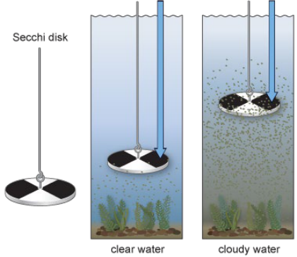
50
Water clarity is typically assessed using a Secchi Disk, as described by the University of
Wisconsin Stevens Point (UWSP, n.d.). This disk, used in Wisconsin, comprises an 8-inch
diameter disk divided into 4 quadrants alternating between white and black (Figure 8). Attached
to a graduated rope and equipped with a bottom weight to maintain horizontal orientation, the
disk is slowly lowered into the water. The process involves marking the point where the disk is
no longer visible by affixing a clothespin on the rope at the water's surface. Subsequently, the
disk is lowered another 2 feet, gradually raised until visible, and marked with a second
clothespin. The Secchi depth recorded is the average between the two markings (WDNR, 2021).
Figure 8 Measuring water clarity with a secchi disk, Image from The Many Faces of Water
(Mierzynski, 2017)
Water clarity data for each lake is collected by volunteers multiple times during the summer
months and is accessible on the WDNR website (WDNR
4
, n.d.). The data utilized in this study
analysis (SecchiDepth) represents the average of all summer-time measurements spanning from
2010 to 2020.
51
3.3.3. Habitat Assessment
The first chapter of this study provides an overview of the Wisconsin Department of Natural
Resources' (WDNR) shoreland habitat assessment. In summary, this assessment utilizes data
from the riparian, bank, and littoral zones to compute a disturbance index for each property.
Properties with higher index values are indicative of greater levels of shoreland disturbance
compared to those with lower values (WDNR, 2023).
This chapter of the study focuses on a lake-level disturbance index (MMI_L) constructed using
shoreland information from all properties surrounding the lake, amalgamating this data to
generate a single index representative of the lake's overall disturbance level (WDNR, 2023).
3.4. Methodology
Regression models were employed to assess whether shoreland disturbances affect water quality,
while controlling for lake characteristics and nearby land use. Five model specifications were
considered. All five followed the general regression equation format represented in equation 6
with the measurement of Secchi depth representing water quality used as the dependent variable.
SD
i
= β
0
+ β
1
X
1
+ β
2
X
2
+ β
3
X
3
+ e Equation 6
Where: SD = Secchi Depth
β = coefficients
X = LULC percents and Lake type
e = error term
In the first model (Model A), Secchi depth (SecchiDepth) was regressed on the percentage of
each land use class in Buffer 1 to examine the relationship between land use classes and water
clarity. Lake depth and lake area were included as independent variables, following the approach
of some hedonic model specifications. Additionally, a factor variable was introduced to

52
distinguish between three different lake types: DRAINAGE, SEEPAGE, and SPRING. As
defined by the WDNR
5
(n.d.), a seepage lake lacks surface inflow or outflow, a drainage lake
experiences surface water flow into and/or out of the lake, and a spring lake, or headwater lake,
receives water from subsurface sources and has a watershed draining less than four square miles
into it. Given that a drainage lake receives surface water inflow, it is expected to exhibit lower
water clarity due to upstream runoff.
The second model (Model B) mirrored Model A, except that it utilized the percentage of each
land use class in Buffer 3. A third model (Model C) regressed SecchiDepth against the lake's
average MMI_L to explore the relationship between variations in shoreland disturbances and
water clarity. Finally, Models D and E were developed by incorporating the MMI_L variable
into the variables used in Models A and B, respectively.
Table 3.2 Regression Model Specifications for Lake Water Clarity Analysis (Dependent
Variable: Secchi Depth)
Model
Secchi
Buffer LULC
MMI_L
Lake Variables
A
x
0-500
x
B
x
500-2500
x
C
x
x
D
x
0-500
x
x
E
x
500-2500
x
x
3.5. Results
This chapter presents the findings from the five regression models (Models A-E), all utilizing the
depth at which the Secchi disk remains visible below the water's surface (SecchiDepth) as the
53
dependent variable. Results from the Secchi depth regressions are detailed in Table 3.3, while
overall model statistics are summarized in Table 3.4.
Model A incorporated land use characteristics within a 500-foot buffer zone surrounding each
lake, along with lake area, lake depth, and indicators for lake type (e.g., seepage, spring). The r
2
value for Model A was 0.4964, with only the lake type and lake depth variables emerging as
significant predictors of lake clarity. Both spring lakes and seepage lakes were associated with
greater Secchi depth measurements relative to drainage lakes, with statistical significance at
p<0.01. Moreover, lake depth exhibited a positive correlation with water clarity, also significant
at p<0.01. Surprisingly, land use variables within the buffer zone were not found to be
significantly related to water clarity, contrary to expectations from previous studies (Zampella et
al., 2007; Parkyn et al., 2003; Garrison et al., 2000).
Model B utilized the same variables as Model A but based land use variables on a buffer zone of
500 – 2500 feet. While the r
2
and adjusted r
2
values increased slightly from 0.4964 and 0.4604 to
0.5041 and 0.4687, respectively, the only significant variables remained the lake characteristics.
Thus, this model did not identify a relationship between land use/land cover (LULC) variables
and water quality.
Model C was a simple linear regression between lake disturbance indices, developed by the
WDNR, and Secchi depth measurement. The r
2
value was 0.0139, indicating minimal
explanation of variation in lake water clarity. Although Figure 9 depicts a positive correlation
between Secchi depth and the level of shoreland disturbance around the lake, this relationship
lacked statistical significance, with a p-value of 0.2082.

54
In Model D, the lake disturbance index variable (MMI_L) was added to Model A. This addition
increased the r
2
value from 0.4964 to 0.5471, a rise of approximately 5.1%. The lake type and
depth variables maintained their positive relationship with lake clarity at a significance level of
p<0.01, with notable changes observed in the LULC variables. Specifically, the percentage of
land covered by tree cover and built area showed a positive and statistically significant
relationship with Secchi depth relative to rangeland area. Although the correlation between tree
cover and water clarity aligned with expectations, the unexpected positive relationship between
built area and water clarity requires further investigation.
Finally, Model E incorporated the MMI_L variable into Model B. Similar to Model D, the
addition of MMI_L increased the r
2
value. This model also demonstrated changes in the LULC
variables, with tree cover and built area being positively and significantly related to water clarity
at p<0.1. However, the disturbance index in both models D and E was not significant, suggesting
its inclusion did not enhance the model's ability to explain variation in water clarity.
Table 3.3 Regression Model Results (Dependent Variable: Secchi Depth)
LULC Class No.
Model A
Buffer 1
Model B
Buffer 3
Model C
Model D
Buffer 1
Model E
Buffer 3
Dependent
Variable
Secchi
Depth
Secchi
Depth
Secchi
Depth
Secchi
Depth
Secchi
Depth
MMI_L
0.0065
(0.2082)
-0.0015
(0.7473)
-0.0003
(0.9463)
Lake Type
SEEPAGE
4.1943***
(0.0000)
4.4460***
(0.0000)
5.1108***
(0.0000)
5.4380***
(0.0000)
Lake Type
SPRING
2.6180***
(0.0017)
2.6955***
(0.0013)
2.3855***
(0.0092)
2.6697***
(0.0036)
Lake Depth
0.1522***
(0.0000)
0.1593***
(0.0000)
0.1527***
(0.0000)
0.1496***
(0.0000)
Lake Area
-0.0007
(0.1674)
-0.0006
(0.1948)
-0.0005
(0.3238)
-0.0004
(0.4366)
1
-0.0238
(0.7486)
0.0276
(0.6179)
-0.0386
(0.6299)
0.0560
(0.3853)

55
2
0.0449
(0.2433)
0.0611
(0.2210)
0.0738*
(0.0548)
0.1033*
(0.0606)
4
-0.0309
(0.7051)
-0.1298
(0.1298)
0.0860
(0.3309)
0.0186
(0.9275)
5
-0.0389
(0.4947)
0.0164
(0.7464)
-0.0170
(0.7722)
0.0557
(0.3161)
7
0.0453
(0.2780)
0.0606
0.3056 ()
0.0745*
(0.0915)
0.1109*
(0.0928)
8
-3.9529
(0.5178)
-0.3200
(0.9689)
13.4740
(0.4605)
1.3658
(0.8636)
Constant
-0.0493
(0.9893)
-2.0135
(0.6646)
8.6602***
(0.0000)
-2.7803
(0.4466)
-6.1124
(0.2252)
Observations
151
151
116
114
114
r
2
0.4964
0.5041
0.0139
0.5633
0.5471
Adjusted r
2
0.4604
0.4687
0.0052
0.5162
0.4983
Note: Robust standard errors reported in parentheses.
*p<0.1; **p<0.05; ***p<0.01
Table 3.4 Overall Model Statistics for Lake Water Clarity Analysis
Statistic
Model A
Model B
Model C
Model D
Model E
Residual Min
-8.4663
-8.0323
-6.4706
-8.1519
-7.9951
Residual 1Q
-2.0847
-1.8789
-3.6508
-1.9495
-1.7434
Residual Median
-0.0126
-0.3231
-0.9313
-0.1601
-0.2434
Residual 3Q
1.7358
1.6264
2.9341
1.5536
1.2433
Residual Max
13.2645
12.5957
11.1883
7.2229
7.2724
Residual
Standard Error
3.3949
3.3688
4.4906
3.1589
3.2168
DF
140
140
114
102
102
F-Stat
13.7992***
14.2318***
1.6020
1109588***
11.2013***
p-value
< 2.2e-16
< 2.2e-16
0.2082
4.233e-14
2.38e-13
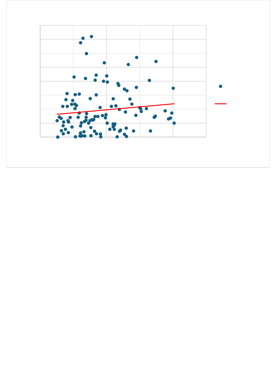
56
Figure 9 Graph of the relationship between the Lakeshore Disturbance Matrix from the Wisconsin
Department of Natural Resources versus the measurement of how deep a secchi disk can be
observed below the surface on 117 Wisconsin lakes.
3.6. Discussion and Conclusion
The study also analyzed if the lakes overall shoreland habitat disturbance value, as assessed by
the WDNR, was a predictor of water clarity, after controlling for the effect of surrounding land
use. Water quality and clarity have been found to affect property values in previous studies (e.g.,
Gibbs et al., 2002; Young, 1984; Moore et al., 2020). In addition, other studies have found that
there is a relationship between LULC and water quality and/or clarity (e.g., Zampella et al.,
2007; Parkyn et al., 2003). The results of this study were not significant for either the LULC or
the MMI_L variables, but additional modeling is warranted.
The study does have several limitations, first is that the study sample size was small relative to
many other HPM analysis. The WDNR studies additional lakes each year, therefore the available
y = 2.1363x + 76.271
R² = 0.0139
0
50
100
150
200
250
300
350
400
0 5 10 15 20 25
Lake Shore Disturbance Matrix
Secchi Depth in feet
Lake Disturbance Matrix vs. Secchi Depth
MMI_L
Trend Line

57
data will continue to grow in the future. But, even with additional data availability from the
WDNR, matching sales data from the MLS is still a limiting factor. Turnover, or sale of these
lakeshore properties is often limited due to the frequency of the properties being passed from
generation to generation without ever becoming for sale in the open market. The study was
further limited by the quality of data available from the MLS, leading to potential omitted
variable bias. MLS data is inputted by real estate agents or their assistants and at times it is
incomplete, or there are errors Many hedonic models have incorporated the age of the property in
the model (Netusil, 2005; Gibbs et al., 2002; Mooney and Eisgruber, 2001), but due to the many
sales records that were missing this information, this variable was not used. Probably more
important that property age would be a variable for property condition, unfortunately property
condition is not an available attribute in MLS data. Condition is important because even very old
properties, that have been extensively remodeled, can be in next to new condition. This study
should be expanded as more information becomes available from both the WDNR and the MLS.
3.7. Future Research
As with the previous chapter, these models should be updated as more data becomes available
from the WDNR. Future research could separate the artificial erosion control disturbance from
the remaining disturbances to evaluate if, as might be expected, they have opposing effects on
water clarity. Additionally, future research could evaluate a broader set of water quality
parameters, such as temperature and phosphorus levels. These additional models may
demonstrate a link between shoreland disturbances and water quality that could inform shoreland
management decisions.
58
4. Conclusion
Compared to some previous hedonic analyses in Wisconsin, this study examines the effects of
shoreland habitat disturbances (the environmental variables) on lakefront housing prices. The
results reveal that certain shoreland disturbances negatively impact property values, while others
are associated with an increase in property value. These mixed findings are expected, as many of
these disturbances offer improved recreational and aesthetic benefits to property owners, despite
their negative effects on shoreland habitat and water quality. It is crucial to acknowledge that
lower water quality can diminish property values.
Shoreland development, in the form of erosion control, beaches, and littoral-zone structures,
provide private benefits to lakeshore property owners, but there is an externality associated with
these features that negatively affects the public good through reduction in overall lake water
quality and aquatic habitat conditions. These private benefits total $36,720 for the average
property in the study sample. Multiplying this by the number of lakeshore properties in
Wisconsin, I estimate $43.5 billion (1.2M x $36,719.82) in benefits to homeowners from
shoreland development features. This estimate should be viewed cautiously as it assumes the
sample properties and lakes are representative of those across the state; nevertheless, it highlights
the considerable value of shoreland development and, conversely, the considerable loss
associated with converting shoreland back to a more natural condition.
Whether it makes economic sense to restore some shoreland areas to a more natural condition
depends on the benefits associated with improved water quality and habitat. Although the second
analysis in this study does not find a statistically significant correlation between water clarity and
shoreland disturbances, there is ample evidence to suggest that natural shoreland reduces
59
pollutant loading and provides critical habitat for fish populations (Munsch et al., 2017). From a
policy perspective, it is necessary to balance the benefit and costs of shoreland development.
To mitigate the impact of shoreland disturbance on the habitat of fish and other aquatic species,
it is imperative for policymakers and regulators to educate the public about conservation efforts
that enhance both water quality and shoreland property values (Munsch et al., 2017). These
actions are particularly viable when they align with both societal goals, such as erosion control
and recreational access, and ecological goals, such as water quality and habitat management.
However, it's essential to recognize that education outreach may have limited impact on
conservation efforts, as many shoreland disturbance features offer substantial non-market
benefits to homeowners.
It is also possible to incentivize homeowners to restore shoreland using subsidies. The WDNR is
currently spending $1.53 million on such subsidies, along with a social media project to educate
property owners on the positive outcomes of a more natural shoreland area. But results from this
study suggest that benefits of shoreland development are substantially greater than the available
subsidies. Estimated WTP from the hedonic analysis could be used to develop more effective set
of subsidies to help property owners transform their shorelines from disturbed, to a more natural
and environmentally friendly shoreland with native plantings.
To establish an efficient subsidy program, it will be necessary for the WDNR to better quantify
the public benefits of shoreland restoration. The WDNR can show the value of the public good
by presenting evidence that more natural shorelands will improve water quality and promote a
more diverse aquatic habitat, which will promote greater fishing opportunities. These changes
will lead to increased recreational, aesthetic, and non-use benefits. By quantifying and
monetizing these benefits, the WDNR can compare the benefits and costs of shoreland
60
restoration. A study in Iowa, for instance, found that the recreational benefits related to water
quality on inland lakes were greater than the cost of lake restoration (Otto et al., 2007). Likewise,
an analysis of benefits of shoreland restoration in Wisconsin, coupled with the WTP values
estimated from this analysis, can be used to evaluate where the benefits of shoreland restoration
are likely to exceed costs to the homeowner.
In conclusion, Wisconsin boasts approximately 15,000 lakes and 1.2 million lakeshore
properties. This hedonic analysis investigates the effects of various shoreland disturbances on
shoreline housing prices. The study demonstrates that shoreland disturbances are linked to higher
property values but also lower lake water quality, as evidenced by other studies showing a
reduction in property values. The findings underscore the importance of evaluating trade-offs
between homeowner preferences for shoreland features (e.g., erosion control, boathouses) and
near-shore water quality and habitat conditions when considering shoreland management
practices.

61
Bibliography
ArcGIS Pro (2023) https://pro.arcgis.com/en/pro-app/latest/tool-reference/spatial-statistics/what-
is-a-z-score-what-is-a-p-value.htm, last access 29 October 2023.
ArcGIS Pro (n.d.) https://pro.arcgis.com/en/pro-app/3.1/tool-reference/spatial-statistics/h-how-
hot-spot-analysis-getis-ord-gi-spatial-stati.htm, last accessed 2 April 2024.
Box, G. E., & Cox, D. R. (1964). An analysis of transformations. Journal of the Royal Statistical
Society Series B: Statistical Methodology, 26(2), 211-243.
Champ, P. A., Boyle, K. J., & Brown, T. C. (Thomas C. (2003). A primer on nonmarket
valuation / edited by Patricia A. Champ, Kevin J. Boyle, and Thomas C. Brown. Kluwer
Academic Publishers.
Clapper, J., & Caudill, S. B. (2014). Water quality and cottage prices in Ontario. Applied
Economics, 46(10), 1122–1126. https://doi.org/10.1080/00036846.2013.851778
Cordell, H. K., & Bergstrom, J. C. (1993). Comparison of recreation use values among
alternative reservoir water level management scenarios. Water resources research, 29(2), 247-
258.
David, E. L. (1968). Lakeshore property values: a guide to public investment in recreation.
Water Resources Research, 4(4), 697-707.
Dziuk, H., & Heiskary, S. (2003). Local economic impact of healthy lakes. LakeLine, 23(3), 21-
23.
Embke, H. S., Douglas Beard Jr, T., Lynch, A. J., & Vander Zanden, M. J. (2020). Fishing for
food: quantifying recreational fisheries harvest in Wisconsin lakes. Fisheries, 45(12), 647-655.
ESRI (2023) Sentinel-2 10m Land Use/Land Cover Time Series
https://livingatlas.arcgis.com/landcoverexplorer/#mapCenter=-
3.286%2C31.34%2C3&mode=step&timeExtent=2017%2C2021&year=2022&downloadMode=t
rue last accessed 26 January 2024
ESRI (n.d.) ArcGIS Pro https://www.esri.com/en-us/arcgis/products/arcgis-pro/overview last
accessed 31 January 2024
FRED (n.d.) Federal Reserve Economic Data https://fred.stlouisfed.org/ last accessed 31 January
2024
Garrison, P. J., & Wakeman, R. S. (2000). Use of paleolimnology to document the effect of lake
shoreland development on water quality. Journal of Paleolimnology, 24, 369-393.

62
Gibbs, J. P., Halstead, J. M., Boyle, K. J., & Huang, J. C. (2002). An hedonic analysis of the
effects of lake water clarity on New Hampshire lakefront properties. Agricultural and Resource
Economics Review, 31(1), 39-46.
Guignet, D., Heberling, M. T., Papenfus, M., & Griot, O. (2022). Property values, water quality,
and benefit transfer: A nationwide meta-analysis. Land economics, 98(2), 191-218.
Heinrich, J., & Kashian, R. (2010). Pricing the Homebuyer’s Proximity to Open Land. The
Journal of Applied Business and Economics, 11(1), 80–.
Horsch, E. J., & Lewis, D. J. (2009). The Effects of Aquatic Invasive Species on Property
Values: Evidence from a Quasi-Experiment. Land Economics, 85(3), 391–409.
https://doi.org/10.3368/le.85.3.391
Huang, W., Mao, J., Zhu, D., & Lin, C. (2020). Impacts of Land Use and Land Cover on Water
Quality at Multiple Buffer-Zone Scales in a Lakeside City. Water (Basel), 12(1), 47-.
https://doi.org/10.3390/w12010047
Jennings, M. J., Emmons, E. E., Hatzenbeler, G. R., Edwards, C., & Bozek, M. A. (2003). Is
Littoral Habitat Affected by Residential Development and Land Use in Watersheds of Wisconsin
Lakes? Lake and Reservoir Management, 19(3), 272–279.
https://doi.org/10.1080/07438140309354092
Jin, D., Hoagland, P., Au, D. K., & Qiu, J. (2015). Shoreline change, seawalls, and coastal
property values. Ocean & Coastal Management, 114, 185-193.
Karra, Kontgis, et al. (2021) “Global land use/land cover with Sentinel-2 and deep learning.”
IGARSS 2021-2021 IEEE International Geoscience and Remote Sensing Symposium. IEEE,
2021.
Kashian, R., & Winden, M. (2020). An Assessment of Lakefront Property Values Based on a
Decline in Water Levels: It’s Impact on Value and Taxes.
Klessig, L. L. (2001). Lakes and society: The contribution of lakes to sustainable societies. Lakes
& Reservoirs: Research & Management, 6(2), 95-101.
Lansford, N. H., & Jones, L. L. (1995). Recreational and Aesthetic Value of Water Using
Hedonic Price Analysis. Journal of Agricultural and Resource Economics, 20(2), 341–355.
https://doi.org/10.22004/ag.econ.30776
Loomis, J., & Feldman, M. (2003). Estimating the benefits of maintaining adequate lake levels to
homeowners using the hedonic property method. Water Resources Research, 39(9).

63
Mamun, S., Castillo-Castillo, A., Swedberg, K., Zhang, J., Boyle, K. J., Cardoso, D., Kling, C.
L., Nolte, C., Papenfus, M., Phaneuf, D., & Polasky, S. (2023). Valuing water quality in the
United States using a national dataset on property values. Proceedings of the National Academy
of Sciences - PNAS, 120(15), e2210417120–e2210417120.
https://doi.org/10.1073/pnas.2210417120
Macbeth, E. J. (1989). The relationship of shoreland zoning elements to the aesthetics of
developed lakeshores in Wisconsin (Doctoral dissertation).
Mierzynski, M. (2017). The Many Faces of Water,
http://www.themanyfacesofwater.eu/index.php/2017/05/19/measuring-water-clarity-with-secchi/
last accessed 1 May 2024
Mooney, S., & Eisgruber, L. (2001). The influence of riparian protection measures on residential
property values: The case of the Oregon Plan for Salmon and Watersheds. The Journal of Real
Estate Finance and Economics, 22(2–3), 273–286. https://doi.org/10.1023/A:1007899716050
Moore, M. R., Doubek, J. P., Xu, H., & Cardinale, B. J. (2020). Hedonic price estimates of lake
water quality: Valued attribute, instrumental variables, and ecological-economic
benefits. Ecological Economics, 176, 106692.
Munsch, S. H., Cordell, J. R., & Toft, J. D. (2017). Effects of shoreline armouring and overwater
structures on coastal and estuarine fish: opportunities for habitat improvement. Journal of
Applied Ecology, 54(5), 1373-1384.
Netusil, N. R. (2005). The effect of environmental zoning and amenities on property values:
Portland, Oregon. Land Economics, 81(2), 227-246.
Nicholls, S., & Crompton, J. L. (2018). The contribution of scenic views of, and proximity to,
lakes and reservoirs to property values. Lakes & Reservoirs: Research & Management, 23(1),
63-78.
Otto, D., Monchuk, D., Jintanakul, K., & Kling, C. (2007). The economic value of Iowa’s natural
resources. Iowa state University.
Papenfus, M. M., & Provencher, B. (2005, November). A hedonic analysis of environmental
zoning: Lake classification in Vilas County, Wisconsin. In Unpublished manuscript, University
of Wisconsin-Madison. Retrieved from http://www. aae. wisc. edu/seminars/papers/2005%
20Fall% 20papers/AppEcon/provencher (Vol. 12).
Parkyn, S. M., Davies‐Colley, R. J., Halliday, N. J., Costley, K. J., & Croker, G. F. (2003).
Planted riparian buffer zones in New Zealand: do they live up to expectations?. Restoration
ecology, 11(4), 436-447.
R (n.d.) The R Project for Statistical Computing https://www.r-project.org/ last accessed 31
January 2024

64
Rahman, R. (2021). Economic Value of Water Quality Improvements in Ontario (Doctoral
dissertation, University of Saskatchewan).
Rosen, S. (1974). Hedonic prices and implicit markets: product differentiation in pure
competition. Journal of political economy, 82(1), 34-55.
Sakia, R. M. (1992). The Box-Cox transformation technique: a review. Journal of the Royal
Statistical Society Series D: The Statistician, 41(2), 169-178.
Schindler, D. W., Armstrong, F. A. J., Holmgren, S. K., & Brunskill, G. J. (1971).
Eutrophication of Lake 227, Experimental Lakes Area, northwestern Ontario, by addition of
phosphate and nitrate. Journal of the Fisheries Board of Canada, 28(11), 1763-1782.
Schnaiberg, J., Riera, J., Turner, M. et al. Explaining Human Settlement Patterns in a
Recreational Lake District: Vilas County, Wisconsin, USA. Environmental Management 30, 24–
34 (2002). https://doi.org/10.1007/s00267-002-2450-z
Sliva, L., & Williams, D. D. (2001). Buffer zone versus whole catchment approaches to studying
land use impact on river water quality. Water research, 35(14), 3462-3472.
Taylor, L. O. (2003). The hedonic method. In A primer on nonmarket valuation (pp. 331-393).
Dordrecht: Springer Netherlands.
Tietenberg, T., & Lewis, L. (2019). Natural resource economics: The essentials. Routledge.
Tobler, W. R. (1970). A computer movie simulating urban growth in the Detroit
region. Economic geography, 46(sup1), 234-240.
Topp, S. N., Pavelsky, T. M., Stanley, E. H., Yang, X., Griffin, C. G., & Ross, M. R. (2021).
Multi-decadal improvement in US lake water clarity. Environmental Research Letters, 16(5),
055025.
UWSP (n.d.) The Secchi Disk and Our Eyes - Working Together To Measure Clarity of Our
Lakes chrome-extension://efaidnbmnnnibpcajpcglclefindmkaj/https://www3.uwsp.edu/cnr-
ap/UWEXLakes/Documents/resources/newsletter/vol31-
vol35/FurtherReading/Secchi%20Article%20-%20Full.pdf last accessed 12 March 2024.
Van Hengstum, P. J., Reinhardt, E. G., Boyce, J. I., & Clark, C. (2007). Changing sedimentation
patterns due to historical land-use change in Frenchman’s Bay, Pickering, Canada: evidence
from high-resolution textural analysis. Journal of Paleolimnology, 37, 603-618.
Walsh, P. (2009). Hedonic property value modeling of water quality, lake proximity, and spatial
dependence in central Florida. University of Central Florida.
WDNR (2023) Shoreland Habitat Disturbance in Wisconsin
https://www.arcgis.com/home/item.html?id=6b5e408d2ecf4b45b9958c9bfab0e607 last accessed
19 October 2023.

65
WDNR (2021) Secchi Disk Monitoring Procedure
https://dnr.wisconsin.gov/topic/SurfaceWater/Monitoring.html last accessed 25 January 2024
WDNR (2020) Lake Shoreland & Shallows Habitat Monitoring Field Protocol
https://dnr.wisconsin.gov/topic/SurfaceWater/Monitoring.html last accessed 23 September 2023
WDNR (2017) Chapter NR 115 https://docs.legis.wisconsin.gov/code/admin_code/nr/100/115
last accessed 19 September 2023
WDNR (2009) Wisconsin Lakes https://dnr.wi.gov/lakes/lakebook/wilakes2009bma.pdf last
accessed 19 September 2023
WDNR
1
(n.d.) Shoreland Habitat Disturbance Viewer
(https://www.arcgis.com/apps/dashboards/e60c681037ff491389dd9199d6427d73 last accessed
29 January 2024
WDNR
2
(n.d.) https://data-wi-dnr.opendata.arcgis.com/search?collection=Dataset last accessed
31 January 2024
WDNR
3
(n.d.) Find A Lake https://apps.dnr.wi.gov/lakes/lakepages/Default.aspx last accessed
31 January 2024
WDNR
4
(n.d.) Surface Water Integrated Monitoring System (SWIMS) Database
https://dnr.wisconsin.gov/topic/SurfaceWater/SWIMS last accessed 31 January 2024
WDNR
5
(n.d.) Wisconsin’s Riverine and Lake Natural Communities
https://dnr.wisconsin.gov/topic/Rivers/NaturalCommunities.html#:~:text=If%20there%20is%20s
urface%20water,classified%20as%20a%20drainage%20lake. Last accessed 2 February 2024
WRA (2024) Wisconsin Realtors Association https://www.wra.org/ last accessed 31 January
2024
Wisconsin State Cartographers Office (n.d.). Statewide Parcel Map Initiative.
https://www.sco.wisc.edu/parcels/data/ last accessed 31 January 2024.
Wolf, D., Klaiber, H. A., & Gopalakrishnan, S. (2022). Beyond marginal: Estimating the demand
for water quality. Resource and Energy Economics, 68, 101299.
Yanggen, D. A., & Kusler, J. A. (1968). Natural resource protection through shoreland
regulation: Wisconsin. Land Economics, 44(1), 73-86.
Young, C. E. (1984). PERCEIVED WATER QUALITY AND THE VALUE OF SEASONAL
HOMES 1. JAWRA Journal of the American Water Resources Association, 20(2), 163-166.
Zampella, R. A., Procopio, N. A., Lathrop, R. G., & Dow, C. L. (2007). Relationship of Land‐
Use/Land‐Cover Patterns and Surface‐Water Quality in The Mullica River Basin 1. JAWRA
Journal of the American Water Resources Association, 43(3), 594-604.

66
Appendix
Table A.1 Robustness Checks for Hedonic Property Model Results (Dependent Variable:
Natural Log of Adjusted Sales Price).
Variable
Model 3
Model 3a
Model 3b
Model3c
Model3d
LnGLA
0.4798***
(0.0000)
0.4827***
(0.0000)
0.5029***
(0.0000)
0.4575***
(0.0000)
0.5172***
(0.0000)
Garage Spaces
0.0657***
(0.000001)
0.0636***
(0.00001)
0.0531***
(0.0024)
0.0645***
(0.000001)
0.0649***
(0.000001)
Total Bath >2
0.1258**
(0.0245)
0.1373**
(0.0281)
0.1344*
(0.0843)
0.1540***
(0.0054)
0.0920
(0.1124)
2
-0.0002
(0.9958)
0.0027
(0.9452)
-0.0029
(0.9519)
0.0225
(0.5279)
-0.0181
(0.6228)
Ln of Lot Acres per GIS
0.0973***
(0.0007)
0.0945***
(0.0028)
0.1010**
(0.0118)
0.1150***
(0.00005)
0.0861***
(0.0033)
Ln of Acres/Shore Length
-0.0916**
(0.0157)
-0.1002**
(0.0142)
-0.0833
(0.1040)
-0.1204***
(0.0014)
-0.0721*
(0.0661)
Manicured Lawn Percent
-0.0002
(0.6354)
0.0001
(0.8755)
0.00005
(0.9436)
-0.0001
(0.9145)
-0.0004
(0.4045)
Canopy Percent
0.0002
(0.5734)
0.0003
(0.4842)
0.0002
(0.7820)
0.0002
(0.7100)
0.0003
(0.5570)
Beach Percent
0.0017*
(0.0314)
0.0019**
(0.0377)
0.0020*
(0.0961)
0.0006
(0.4483)
0.0020**
(0.0133)
Structures Lit Zone
0.0296**
(0.0128)
0.0233*
(0.0781)
0.0082
(0.6268)
0.0235**
(0.0441)
0.0339***
(0.0056)
Structures Rip Zone
-0.0052
(0.4819)
-0.0075
(0.3628)
-0.0085
(0.4178)
-0.0072
(0.3142)
-0.0055
(0.4632)
Erosion Control Percent
0.0012***
(0.0018)
0.0009**
(0.0350)
0.0011**
(0.0311)
0.0011***
(0.0028)
-0.1216***
(0.0092)
Erosion Present
-0.1138**
(0.0120)
-0.1127**
(0.0206)
-0.1310**
(0.0235)
-0.0551
(0.2253)
-0.1216***
(0.0092)
Bypass_Pres
-0.00051
(0.6063)
-0.0063
(0.5855)
-0.0090
(0.5255)
-0.0053
(0.5829)
-0.0008
(0.9391)
Vegetation Present
0.0210
(0.5020)
0.0418
(0.2339)
0.0356
(0.4244)
0.0282
(0.3593)
0.0093
(0.7756)
Vegetation Removed
-0.0084
(0.8373)
0.0060
(0.8951)
-0.0156
(0.7891)
-0.0148
(0.7135)
-0.0095
(0.8223)
Constant
8.8934***
(0.0000)
8.7032***
(0.0000)
8.4864***
(0.0000)
8.9000***
(0.0000)
8.6952***
(0.0000)
Year fixed effect
Yes
Yes
Yes
Yes
Yes
Quarter fixed effect
Yes
Yes
Yes
Yes
Yes
Lake fixed effect
Yes
Yes
Yes
Yes
Yes
School District fixed effect
No
No
No
Yes
No
Observations
847
681
463
847
802
r
2
0.6270
0.6306
0.6377
0.6445
0.6157
Adjusted r
2
0.5769
0.5735
0.5607
0.5946
0.5608
Note: Robust standard errors reported in parentheses.
*p<0.1; **p<0.05; ***p<0.01
